GeoWave Quickstart Guide
The GeoWave quickstart guide is designed to allow a new user to run through a few simple use cases with the GeoWave framework using the Command-Line Interface. While this guide uses a local key/value store, a version of the guide is available here which utilizes EMR on AWS.
Preparation
Install GeoWave
This guide assumes that GeoWave has already been installed and is available on the command-line. See the Installation Guide for help with the installation process.
| Several commands used in this guide are only available if GeoWave was installed using the standalone installer. |
Create Working Directory
In order to keep things organized, create a directory on your system that can be used throughout the guide. The guide will refer to this directory as the working directory.
$ mkdir quickstart
$ cd quickstart
Download Sample Data
We will be using data from the GDELT Project in this guide. For more information about the GDELT Project please visit their website here.
Download one or more ZIP files from the GDELT Event Repository into a new gdelt_data folder in the working directory. The examples in this guide will use all of the data from February 2016 (files with a 201602 prefix).
Download Styles
Later in the guide, we will be visualizing some data using GeoServer. For this, we will be using some styles that have been created for the demo.
Download the following styles to your working directory:
When finished, you should have a directory structure similar to the one below.
quickstart
|- KDEColorMap.sld
|- SubsamplePoints.sld
|- gdelt_data
|  |- 20160201.export.CSV.zip
|  |- 20160202.export.CSV.zip
|  |- 20160203.export.CSV.zip
|  |- 20160204.export.CSV.zip
.
.
.
After all the data and styles have been downloaded, we can continue.
Vector Demo
|
Before starting the vector demo, make sure that your working directory is the current active directory in your command-line tool. |
Configure GeoWave Data Store
For this quickstart guide, we will be using RocksDB as the key/value store backend for GeoWave. This is mainly for simplicity, as RocksDB does not require any external services to be made available.
$ geowave store add -t rocksdb --gwNamespace geowave.gdelt --dir . gdeltThis command adds a connection to a RocksDB data store in the current directory under the name gdelt for use in future commands. It configures the connection to put all data for this named store under the geowave.gdelt namespace. After executing the command, the database is not automatically created. Instead, GeoWave will only create a new RocksDB database using this configuration when a command is executed that makes a modification to the data store.
Add an Index
Before ingesting any data, we need to create an index that describes how the data will be stored in the key/value store. For this example we will create a simple spatial index.
$ geowave index add -t spatial gdelt gdelt-spatialThis command adds a spatial index to the gdelt data store with an index name of gdelt-spatial. This is the name that we will use to reference this index in future commands.
Ingest Data
GeoWave has many commands that facilitate ingesting data into a GeoWave data store. For this example, we want to ingest GDELT data from the local file system, so we will use the ingest localToGW command. We will use a bounding box that roughly surrounds Germany to limit the amount of data ingested for the example.
$ geowave ingest localToGW -f gdelt --gdelt.cql "BBOX(geometry,5.87,47.2,15.04,54.95)" ./gdelt_data gdelt gdelt-spatialThis command specifies the input format as GDELT using the -f option, filters the input data using a CQL bounding box filter, and specifies the input directory for all of the files. Finally, we tell GeoWave to ingest the data to the gdelt-spatial index in the gdelt data store. GeoWave creates an adapter for the new data with the type name gdeltevent, which we can use to refer to this data in other commands. The ingest should take about 3-5 minutes.
Query the Data
Now that the data has been ingested, we can make queries against it. The GeoWave programmatic API provides a large variety of options for issuing queries, but for the purposes of this guide, we will use the query language support that is available for vector data. This query language provides a simple way to perform some of the most common types of queries using a well-known syntax. To demonstrate this, perform the following query:
$ geowave query gdelt "SELECT * FROM gdeltevent LIMIT 10"This command tells GeoWave to select all attributes from the gdeltevent type in the gdelt data store, but limits the output to 10 features. After running this command, you should get a result that is similar to the following:
+-------------------------+-----------+------------------------------+----------+-----------+----------------+----------------+-------------+-------------------------------------------------------------------------------------------------------+
| geometry                | eventid   | Timestamp                    | Latitude | Longitude | actor1Name     | actor2Name     | countryCode | sourceUrl                                                                                             |
+-------------------------+-----------+------------------------------+----------+-----------+----------------+----------------+-------------+-------------------------------------------------------------------------------------------------------+
| POINT (15.0395 50.1904) | 510693819 | Thu Feb 11 00:00:00 EST 2016 | 50.1904  | 15.0395   | CZECH          | THAILAND       | EZ          | http://praguemonitor.com/2016/02/11/czech-zoo-acquires-rare-douc-langur-monkeys                       |
| POINT (15.0395 50.1904) | 510694920 | Thu Feb 11 00:00:00 EST 2016 | 50.1904  | 15.0395   | THAILAND       | CZECH          | EZ          | http://praguemonitor.com/2016/02/11/czech-zoo-acquires-rare-douc-langur-monkeys                       |
| POINT (14.7186 50.4983) | 508121628 | Wed Feb 03 00:00:00 EST 2016 | 50.4983  | 14.7186   |                | LEBANON        | EZ          | http://praguemonitor.com/2016/02/03/plane-pick-five-czechs-leave-lebanon-wednesday                    |
| POINT (14.7186 50.4983) | 508121971 | Wed Feb 03 00:00:00 EST 2016 | 50.4983  | 14.7186   | POLICE         |                | EZ          | http://praguemonitor.com/2016/02/03/plane-pick-five-czechs-leave-lebanon-wednesday                    |
| POINT (14.7186 50.4983) | 508122060 | Wed Feb 03 00:00:00 EST 2016 | 50.4983  | 14.7186   | CZECH          |                | EZ          | http://praguemonitor.com/2016/02/03/plane-pick-five-czechs-leave-lebanon-wednesday                    |
| POINT (14.7186 50.4983) | 508122348 | Wed Feb 03 00:00:00 EST 2016 | 50.4983  | 14.7186   | FOREIGN MINIST | LEBANON        | EZ          | http://praguemonitor.com/2016/02/03/plane-pick-five-czechs-leave-lebanon-wednesday                    |
| POINT (14.7186 50.4983) | 508122668 | Wed Feb 03 00:00:00 EST 2016 | 50.4983  | 14.7186   | LEBANON        |                | EZ          | http://praguemonitor.com/2016/02/03/plane-pick-five-czechs-leave-lebanon-wednesday                    |
| POINT (14.7186 50.4983) | 508122669 | Wed Feb 03 00:00:00 EST 2016 | 50.4983  | 14.7186   | LEBANON        |                | EZ          | http://praguemonitor.com/2016/02/03/plane-pick-five-czechs-leave-lebanon-wednesday                    |
| POINT (14.7186 50.4983) | 508122679 | Wed Feb 03 00:00:00 EST 2016 | 50.4983  | 14.7186   | LEBANON        | FOREIGN MINIST | EZ          | http://praguemonitor.com/2016/02/03/plane-pick-five-czechs-leave-lebanon-wednesday                    |
| POINT (14.7186 50.4983) | 508579066 | Thu Feb 04 00:00:00 EST 2016 | 50.4983  | 14.7186   | CZECH          | MEDIA          | EZ          | http://www.ceskenoviny.cz/zpravy/plane-with-five-czechs-flying-from-beirut-to-prague-ministry/1311188 |
+-------------------------+-----------+------------------------------+----------+-----------+----------------+----------------+-------------+-------------------------------------------------------------------------------------------------------+
We can see right away that these results are tagged with the country code EZ which falls under Czech Republic. Since our area of interest is around Germany, perhaps we want to only see events that are tagged with the GM country code. We can do this by adding a WHERE clause to the query.
$ geowave query gdelt "SELECT * FROM gdeltevent WHERE countryCode='GM' LIMIT 10"Now the results show only events that have the GM country code.
+-------------------------+-----------+------------------------------+----------+-----------+------------+------------+-------------+---------------------------------------------------------------------------------------------------------------------------+
| geometry                | eventid   | Timestamp                    | Latitude | Longitude | actor1Name | actor2Name | countryCode | sourceUrl                                                                                                                 |
+-------------------------+-----------+------------------------------+----------+-----------+------------+------------+-------------+---------------------------------------------------------------------------------------------------------------------------+
| POINT (13.0333 47.6333) | 508836788 | Fri Feb 05 00:00:00 EST 2016 | 47.6333  | 13.0333   | GERMANY    |            | GM          | http://www.thespreadit.com/gold-bar-lake-keep-69589/                                                                      |
| POINT (13.0333 47.6333) | 508836797 | Fri Feb 05 00:00:00 EST 2016 | 47.6333  | 13.0333   | GERMANY    | ALBERT     | GM          | http://www.thespreadit.com/gold-bar-lake-keep-69589/                                                                      |
| POINT (13.0333 47.6333) | 508837466 | Fri Feb 05 00:00:00 EST 2016 | 47.6333  | 13.0333   | ALBERT     | GERMANY    | GM          | http://www.thespreadit.com/gold-bar-lake-keep-69589/                                                                      |
| POINT (12.9 47.7667)    | 508569746 | Thu Feb 04 00:00:00 EST 2016 | 47.7667  | 12.9      |            | GERMAN     | GM          | http://www.ynetnews.com/articles/0,7340,L-4762071,00.html                                                                 |
| POINT (12.9 47.7667)    | 508574449 | Thu Feb 04 00:00:00 EST 2016 | 47.7667  | 12.9      | COMPANY    | GOVERNMENT | GM          | http://www.i24news.tv/en/news/international/101671-160204-holocaust-survivors-sue-hungary-for-deportation-of-500-000-jews |
| POINT (12.9 47.7667)    | 508665355 | Thu Feb 04 00:00:00 EST 2016 | 47.7667  | 12.9      | HUNGARY    | GERMANY    | GM          | http://www.jns.org/news-briefs/2016/2/4/14-holocaust-survivors-sue-hungary-in-us-court                                    |
| POINT (12.9 47.7667)    | 508773863 | Fri Feb 05 00:00:00 EST 2016 | 47.7667  | 12.9      |            | GERMAN     | GM          | http://jpupdates.com/2016/02/04/14-holocaust-survivors-sue-hungary-in-u-s-court/                                          |
| POINT (12.9 47.7667)    | 508775266 | Fri Feb 05 00:00:00 EST 2016 | 47.7667  | 12.9      | HUNGARY    | GERMANY    | GM          | http://jpupdates.com/2016/02/04/14-holocaust-survivors-sue-hungary-in-u-s-court/                                          |
| POINT (12.9 47.7667)    | 509245139 | Sat Feb 06 00:00:00 EST 2016 | 47.7667  | 12.9      |            | GERMAN     | GM          | https://theuglytruth.wordpress.com/2016/02/06/hungary-holocaust-survivors-sue-hungarian-government/                       |
| POINT (12.9 47.7667)    | 509327879 | Sun Feb 07 00:00:00 EST 2016 | 47.7667  | 12.9      |            | LARI       | GM          | http://blackgirllonghair.com/2016/02/the-black-victims-of-the-holocaust-in-nazi-germany/                                  |
+-------------------------+-----------+------------------------------+----------+-----------+------------+------------+-------------+---------------------------------------------------------------------------------------------------------------------------+
If we wanted to see how many events belong to to the GM country code, we can perform an aggregation query.
$ geowave query gdelt "SELECT COUNT(*) FROM gdeltevent WHERE countryCode='GM'"+----------+ | COUNT(*) | +----------+ | 81897 | +----------+
We can also perform multiple aggregations on the same data in a single query. The following query counts the number of entries that have set actor1Name and how many have set actor2Name.
$ geowave query gdelt "SELECT COUNT(actor1Name), COUNT(actor2Name) FROM gdeltevent"+-------------------+-------------------+ | COUNT(actor1Name) | COUNT(actor2Name) | +-------------------+-------------------+ | 93750 | 80608 | +-------------------+-------------------+
We can also do bounding box aggregations. For example, if we wanted to see the bounding box of all the data that has HUNGARY set as the actor1Name, we could do the following:
$ geowave query gdelt "SELECT BBOX(*), COUNT(*) AS total_events FROM gdeltevent WHERE actor1Name='HUNGARY'"+------------------------------------------+--------------+ | BBOX(*) | total_events | +------------------------------------------+--------------+ | Env[6.1667 : 14.7174, 47.3333 : 53.5667] | 408 | +------------------------------------------+--------------+
|
In these examples each query was output to console, but there are options on the command that allow the query results to be output to several formats, including geojson, shapefile, and CSV. |
For more information about vector queries, see the queries section of the User Guide.
Kernel Density Estimation (KDE)
We can also perform analytics on data that has been ingested into GeoWave. In this example, we will perform the Kernel Density Estimation (KDE) analytic.
$ geowave analytic kdespark --featureType gdeltevent -m local --minLevel 5 --maxLevel 26 --coverageName gdeltevent_kde gdelt gdeltThis command tells GeoWave to perform a Kernel Density Estimation using a local spark cluster on the gdeltevent type. It specifies that the KDE should be run at zoom levels 5-26 and that the new raster generated should be under the type name gdeltevent_kde. Finally, it specifies the input and output data store as our gdelt store. It is possible to output the results of the KDE to a different data store, but for this demo, we will use the same one. The KDE can take 5-10 minutes to complete due to the size of the dataset.
Visualizing the Data
Now that we have prepared our vector and KDE data, we can visualize it by using the GeoServer plugin. GeoWave provides an embedded GeoServer with the command-line tools.
Run GeoServer
|
Execute the following command in a new terminal window. This command is only available if GeoWave was installed using the standalone installer with the |
$ geowave gs runAfter a few moments, GeoServer should be available by browsing to localhost:8080/geoserver. The login credentials for this embedded service are username admin and password geoserver. The server will remain running until the command-line process is exited. You can exit the process by pressing Ctrl+C or by closing the terminal window.
|
RocksDB only supports a single connection to the database, because of this, you will be unable to perform queries or other data store operations with the CLI while GeoServer maintains a connection to it. If you would like the capability to do both simultaneously, you can use one of the other standalone data stores that are packaged with GeoWave. |
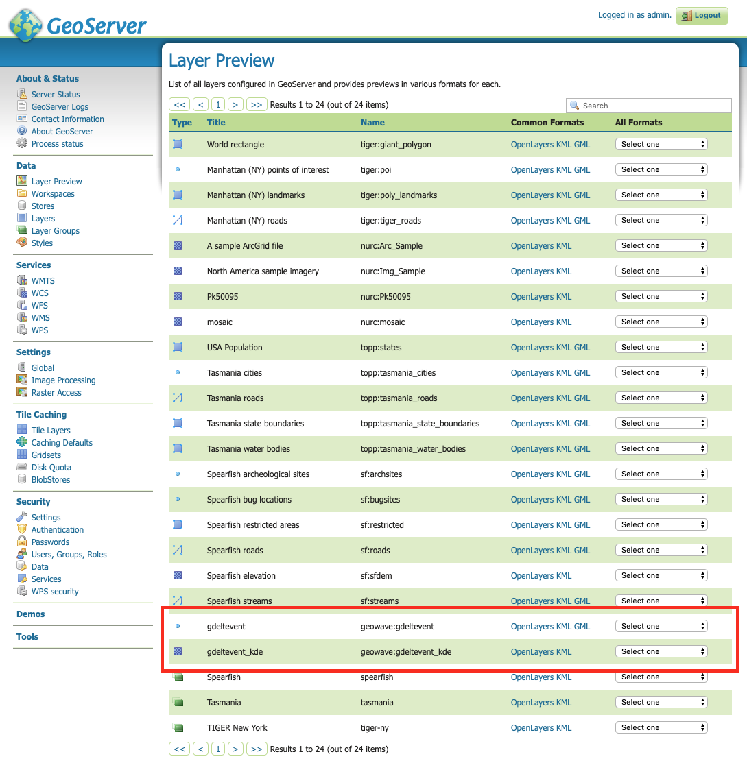
Add Layers
GeoWave provides commands that make adding layers to a GeoServer instance a simple process. In this example, we can add both the gdeltevent and gdeltevent_kde types to GeoServer with a single command.
$ geowave gs layer add gdelt --add allThis command tells GeoWave to add all raster and vector types from the gdelt data store to GeoServer.
Add Styles
We already downloaded the styles that we want to use to visualize our data as part of the preparation step. The KDEColorMap style will be used for the heatmap produced by the KDE analytic. The SubsamplePoints style will be used to efficiently render the points from the gdeltevent type. All we need to do is add them to GeoServer.
$ geowave gs style add kdecolormap -sld KDEColorMap.sld
$ geowave gs style add SubsamplePoints -sld SubsamplePoints.sld
Now we can update our layers to use these styles.
$ geowave gs style set gdeltevent_kde --styleName kdecolormap
$ geowave gs style set gdeltevent --styleName SubsamplePoints
View the Layers
The GeoServer web interface can be accessed in your browser:
Login to see the layers.
-
Username: admin
-
Password: geoserver
Select "Layer Preview" from the menu on the left side. You should now see our two layers in the layer list.
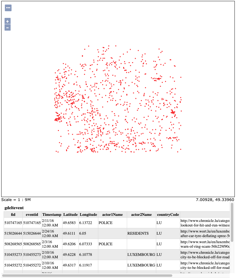
Click on the OpenLayers link by any of these layers to see them in an interactive map.
gdeltevent - Shows all of the GDELT events in a bounding box around Germany as individual points. Clicking on the map preview will show you the feature data associated with the clicked point.
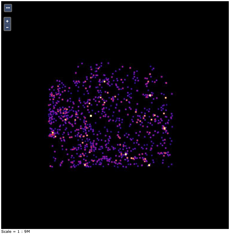
gdeltevent Layergdeltevent_kde - Shows the heat map produced by the KDE analytic in a bounding box around Germany.
|
For this screenshot, the background color of the preview was set to black by appending |
gdeltevent_kde LayerRaster Demo (deprecated)
DISCLAIMER: It appears in March 2022 AWS completely removed LandSat8 Open Data Imagery, effectively deprecating this raster demo In this demo, we will be looking at Band 8 of Landsat raster data around Berlin, Germany. See USGS.gov for more information about Landsat 8.
Install GDAL
The Landsat 8 extension for GeoWave utilizes GDAL (Geospatial Data Abstraction Library), an image processing library, to process raster data. In order to use GDAL, native libraries need to be installed on the system. More info on GDAL can be found here.
GeoWave provides a way to install GDAL libraries with the following command:
$ geowave raster installgdalConfigure GeoWave Data Stores
|
Before continuing the demo, make sure that your working directory is the current active directory in your command-line tool. |
For this demo, we will be using two data stores. One will be used for vector data, and the other will be used for raster data. We will again be using RocksDB for the backend.
$ geowave store add -t rocksdb --gwNamespace geowave.landsatraster --dir . landsatraster
$ geowave store add -t rocksdb --gwNamespace geowave.landsatvector --dir . landsatvector
These commands create two data stores, landsatraster and landsatvector in the current directory.
Add an Index
Before ingesting our raster data, we will add a spatial index to both of the data stores.
$ geowave index add -t spatial -c EPSG:3857 landsatraster spatial-idx
$ geowave index add -t spatial -c EPSG:3857 landsatvector spatial-idx
This is similar to the command we used to add an index in the vector demo, but we have added an additional option to specify the Coordinate Reference System (CRS) of the data. Geospatial data often uses a CRS that is tailored to the area of interest. This can be a useful option if you want to use a CRS other than the default. After these commands have been executed, we will have spatial indices named spatial-idx on both data stores.
Analyze Available Data
We can now see what Landsat 8 data is available for our area of interest.
$ geowave util landsat analyze --nbestperspatial true --nbestscenes 1 --usecachedscenes true --cql "BBOX(shape,13.0535,52.3303,13.7262,52.6675) AND band='B8' AND cloudCover>0" -ws ./landsatThis command tells GeoWave to analyze the B8 band of Landsat raster data over a bounding box that roughly surrounds Berlin, Germany. It prints out aggregate statistics for the area of interest, including the average cloud cover, date range, number of scenes, and the size of the data. Data for this operation is written to the landsat directory (specified by the -ws option), which can be used by the ingest step.
Ingest the Data
Now that we have analyzed the available data, we are ready to ingest it into our data stores.
$ geowave util landsat ingest --nbestperspatial true --nbestscenes 1 --usecachedscenes true --cql "BBOX(shape,13.0535,52.3303,13.7262,52.6675) AND band='B8' AND cloudCover>0" --crop true --retainimages true -ws ./landsat --vectorstore landsatvector --pyramid true --coverage berlin_mosaic landsatraster spatial-idxThere is a lot to this command, but you’ll see that it’s quite similar to the analyze command, but with some additional options. The --crop option causes the raster data to be cropped to our CQL bounding box. The --vectorstore landsatvector option specifies the data store to put the vector data (scene and band information). The --pyramid option tells GeoWave to create an image pyramid for the raster, this is used for more efficient rendering at different zoom levels. The --coverage berlin_mosaic option tells GeoWave to use berlin_mosaic as the type name for the raster data. Finally, we specify the output data store for the raster, and the index to store it on.
Visualizing the Data
We will once again use GeoServer to visualize our ingested data.
Run GeoServer
GeoServer should still be running from the previous demo, but if not, go ahead and start it up again from a new terminal window.
$ geowave gs runAdd Layers
Just like with the vector demo, we can use the GeoWave CLI to add our raster data to GeoServer. We will also add the vector metadata from the vector data store.
$ geowave gs layer add landsatraster --add all
$ geowave gs layer add landsatvector --add all
View the Layers
When we go back to the Layer Preview page in GeoServer, we will see three new layers, band, berlin_mosaic, and scene.
Click on the OpenLayers link by any of these layers to see them in an interactive map.
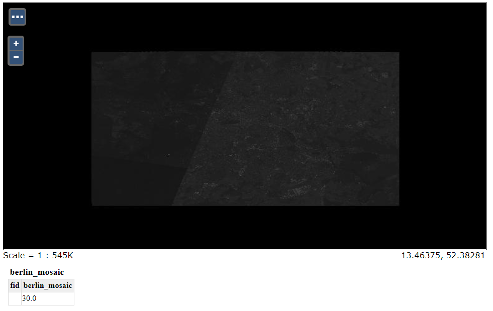
berlin_mosaic - Shows the mosaic created from the raster data that fit into our specifications. This mosaic is made of 5 images.
berlin_mosaic Layerband/scene - Shows representations of the vector data associated with the images. The band and scene layers are identical in this demo.
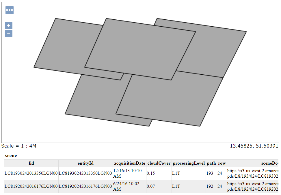
band and scene Layers