GeoWave Overview
Introduction
What is GeoWave
GeoWave is an open-source library to store, index, and search multi-dimensional data in sorted key/value stores. It includes implementations that support OGC spatial types (up to 3 dimensions), and both bounded and unbounded temporal values. Both single and ranged values are also supported in all dimensions. GeoWave’s geospatial support is built on top of the GeoTools project extensibility model. This means that it can integrate natively with any GeoTools-compatible project, such as GeoServer and UDig, and can ingest GeoTools compatible data sources.
Basically, GeoWave is working to bridge geospatial software with distributed computing systems and attempting to do for distributed key/value stores what PostGIS does for PostgreSQL.
Capabilities
-
Add multi-dimensional indexing capability to key/value stores
-
Add support for geographic objects and geospatial operators to key/value stores
-
Provide a GeoServer plugin to allow geospatial data from key/value stores to be shared and visualized via OGC standard services
-
Provide Map-Reduce input and output formats for distributed processing and analysis of geospatial data
Origin
GeoWave was initially developed at the National Geospatial-Intelligence Agency (NGA) in collaboration with RadiantBlue Technologies and Booz Allen Hamilton. The government has unlimited rights and is releasing this software to increase the impact of government investments by providing developers with the opportunity to take things in new directions. The software use, modification, and distribution rights are stipulated within the Apache 2.0 license.
Design Principles
Scalable
GeoWave is designed to operate either in a single-node setup or it can scale out as large as needed to support the amount of data and/or processing resources necessary. By utilizing distributed computing clusters and server-side fine grain filtering, GeoWave is fully capable of performing interactive time and/or location specific queries on datasets containing billions of features with 100 percent accuracy.
Pluggable Backend
GeoWave is intended to be a multi-dimensional indexing layer that can be added on top of any sorted key/value store. Accumulo was chosen as the initial target architecture and support for several other backends have been added over time. In practice, any data store which allows prefix based range scans should be straightforward to implement as an extension to GeoWave.
Modular Framework
The GeoWave architecture is designed to be extremely extensible with most of the functionality units defined by interfaces. GeoWave provides default implementations of these interfaces to cover most use cases, but it also allows for easy feature extension and platform integration – bridging the gap between distributed technologies and minimizing the learning curve for developers. The intent is that the out-of-the-box functionality should satisfy 90% of use cases, but the modular architecture allows for easy feature extension as well as integration into other platforms.
Self-Describing Data
GeoWave stores the information needed to manipulate data, such as configuration and format, in the database itself. This allows software to programmatically interrogate all the data stored in a single or set of GeoWave instances without needing bits of configuration from clients, application servers, or other external stores.
Overview
For many GeoWave users, the primary method of interfacing with GeoWave is through the various Command-Line Interface (CLI) commands. Users will use GeoWave to store, index, or query multi-dimensional data in a key/value store.

Usage typically involves these steps:
-
Configure Data Store
Configure GeoWave to connect to a key/value store.
-
Create Indices
Create one or more indices on the configured data store.
-
Ingest Data
Ingest data into one or more indices on the data store.
-
Process Data
Process data using a distributed processing engine (e.g. MapReduce, Spark).
-
Query/Discover
Query or discover ingested or transformed data using a GeoWave interface. A common interface for exploring GeoWave data is GeoServer, which interfaces with GeoWave through a plugin to visualize geospatial data in the underlying key/value store.
Key Components
Data Stores
A GeoWave data store is the sum of all parts required to make GeoWave function. This includes metadata, statistics, indices, and adapters. GeoWave data stores are typically accessed using a set of configuration parameters that define how to connect to the underlying key/value store. When using the Command-Line Interface (CLI), these configuration parameters are saved locally under a single store name that can be used in future CLI operations.
Indices
A GeoWave index serves as a template that GeoWave uses to store and retrieve data from the key/value store efficiently with a given set of dimensions. Each index can have data from any number of adapters, as long as those adapters conform to the dimensions used by the index. For example, a spatial-temporal index wouldn’t be able to properly index data without a time component, but a spatial-only index would be able to index spatial-temporal data without taking advantage of the time component.
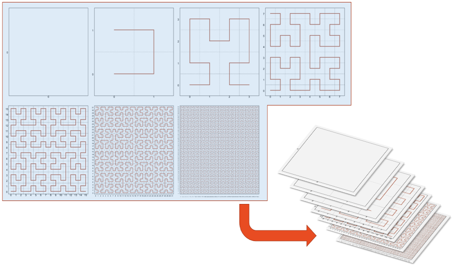
GeoWave uses tiered, gridded, space-filling curves (SFCs) to index data into key/value stores. The indexing information is stored in a generic key structure that can also be used for server-side processing. This architecture allows query, processing, and rendering times to be reduced by multiple orders of magnitude. For a more in-depth explanation of space-filling curves and why they are used in GeoWave indexing, see the theory section of the Developer Guide.
Each index is assigned a name when it is created. This index name is used to reference the index in GeoWave operations.
Adapters/Data Types
In order to handle a multitude of input data types, an adapter is needed to describe the input data type so that can be translated to a format that GeoWave understands. Among others, GeoWave provides a data adapter implementation that supports SimpleFeatures by default, which should cover most use cases for vector data.
An example of this would be if a user had a shapefile and wanted to ingest it into GeoWave. During the ingest process, an adapter would be created to describe and translate all of the fields for each feature in the shapefile so that GeoWave could index and store the data in an optimized format. When that data is read by the user in the future, the adapter would be used to transform the GeoWave data back into SimpleFeature data.
Data that has been added to GeoWave with an adapter is often referred to as a type. Each type has a name that can be used to interact with the data. Throughout the documentation, this name is referred to as a type name.
In GeoWave, the terms adapter and type are often interchangeable.
Statistics
Because GeoWave often deals with large amounts of data, it can be costly to calculate statistics information about a data set. To address this problem, GeoWave has a statistics store that can be configured to keep track of statistics on indices, data types, and fields that can be queried without having to traverse the entire data set. GeoWave provides a number of statistics out of the box that should address a majority of use cases. Some of these include:
-
Ranges over an attribute, including time
-
Enveloping bounding box over all geometries
-
Cardinality of the number of stored items
-
Histograms over the range of values for an attribute
-
Cardinality of discrete values of an attribute
Statistics are generally updated during ingest and deletion. However, due to their nature, range and bounding box statistics are not updated during deletion and may require recalculation. These are the circumstances where recalculation of statistics is recommended:
-
As items are removed from an index, the range and envelope statistics may lose their accuracy if the removed item contains an attribute that represents the minimum or maximum value for the population.
-
When a statistic algorithm is changed, the existing statistic data may not accurately represent the updated algorithm.
Example Screenshots
The screenshots below are of data loaded from various attributed data sets into a GeoWave instance, processed (in some cases) by a GeoWave analytic process, and rendered by GeoServer.
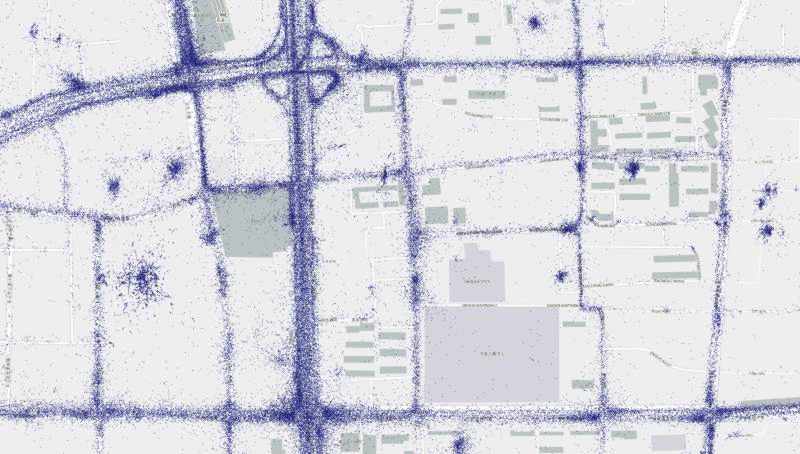
GeoLife
Microsoft research has made available a trajectory data set that contains the GPS coordinates of 182 users over a three year period (April 2007 to August 2012). There are 17,621 trajectories in this data set.
More information on this data set is available at Microsoft Research GeoLife page.

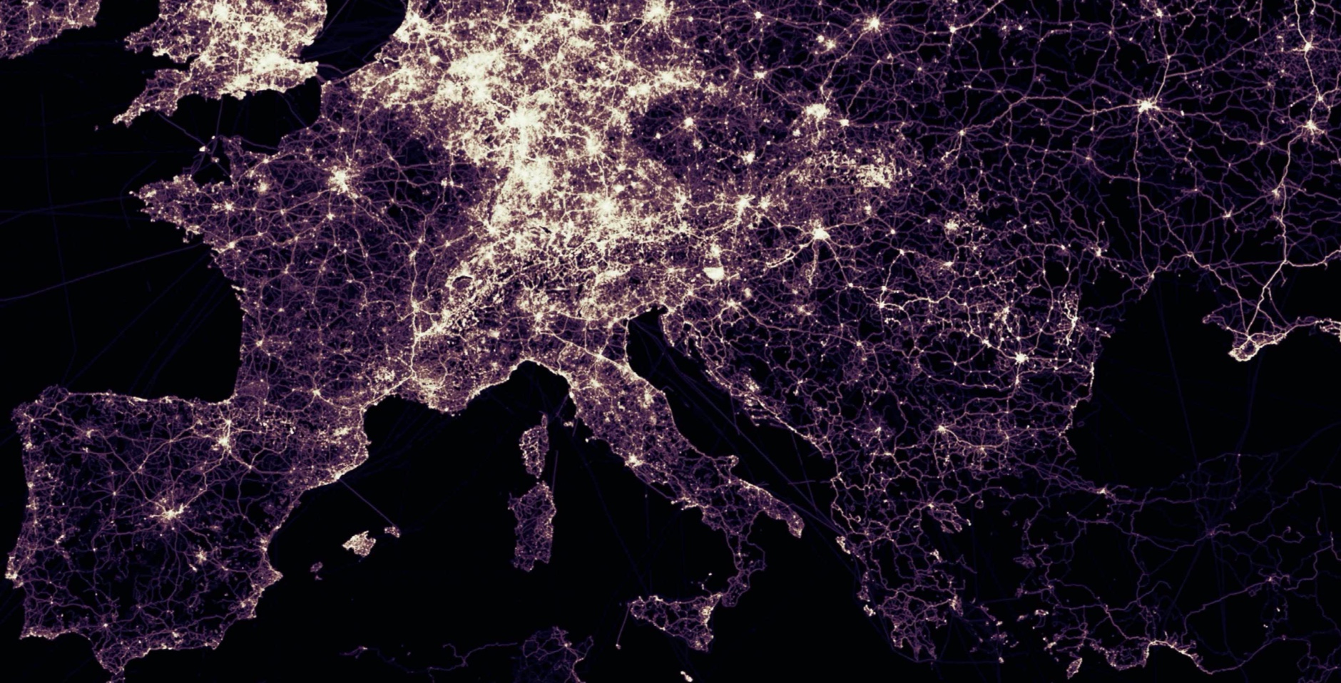
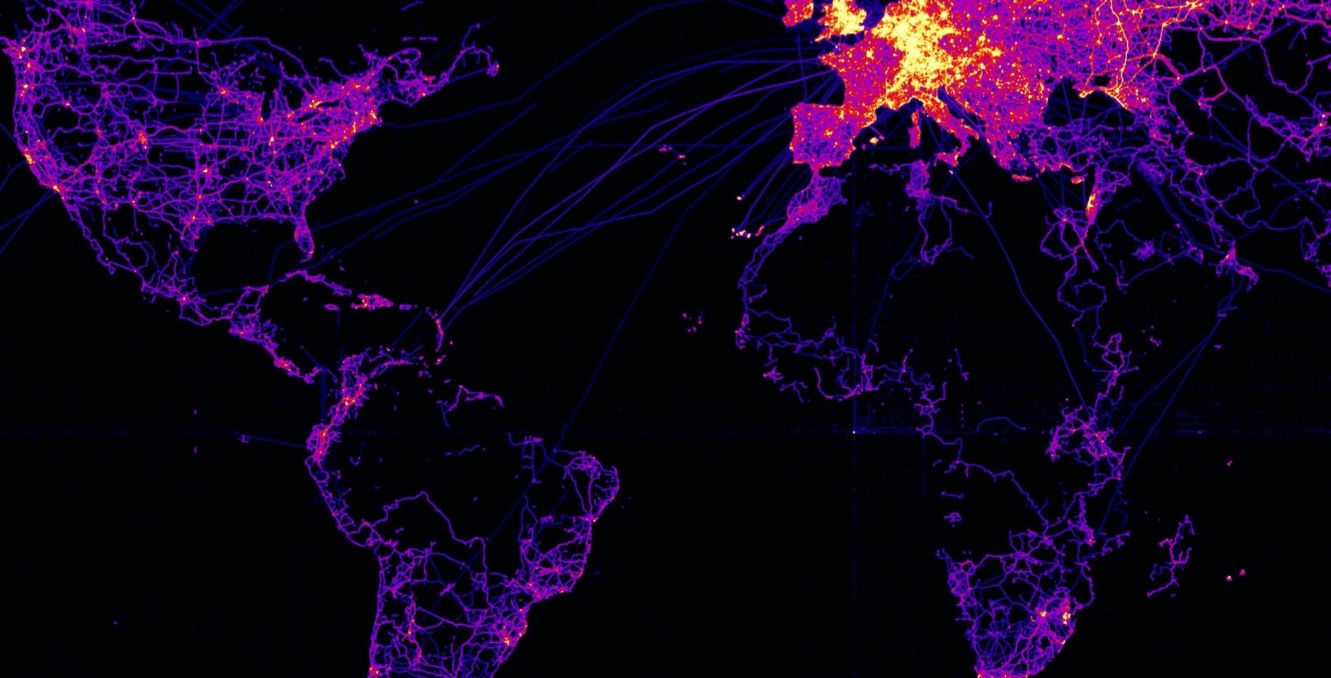
OpenStreetMap GPX Tracks
The OpenStreetMap Foundation has released a large set of user contributed GPS tracks. These are about eight years of historical tracks. The data set consists of just under three billion (not trillion as some websites claim) points, or just under one million trajectories.
More information on this data set is available at GPX Planet page.
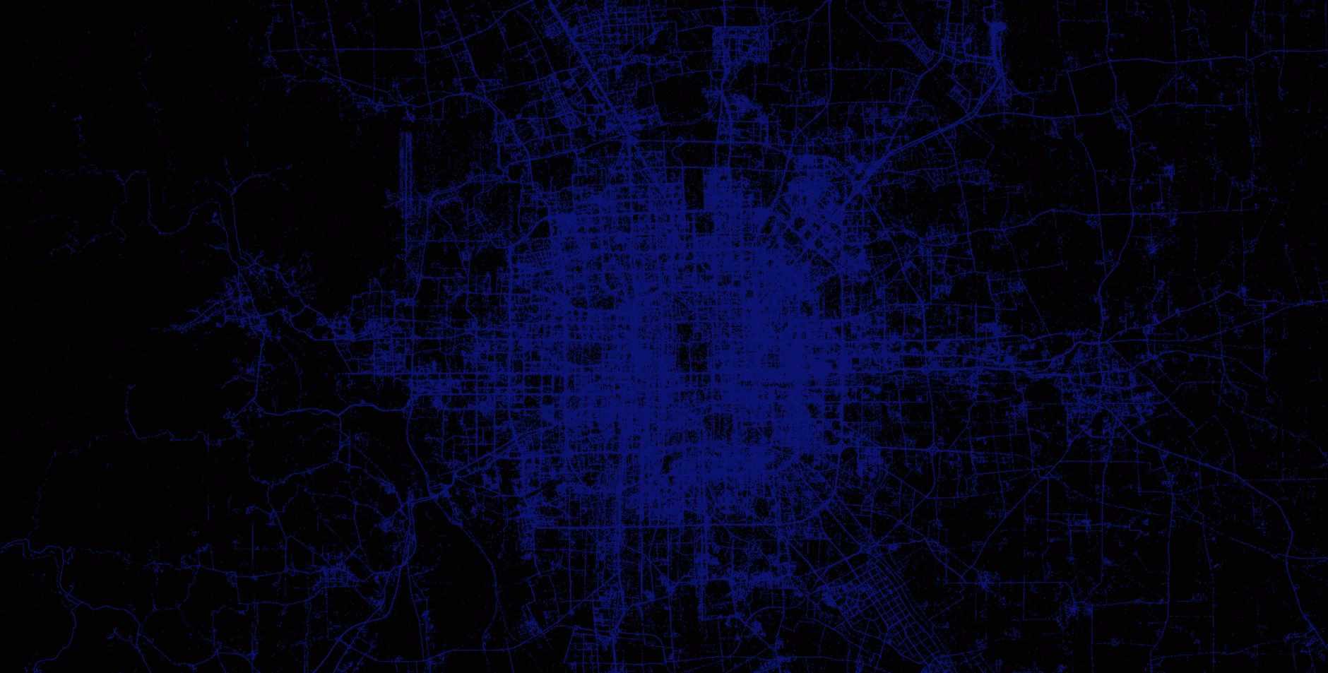
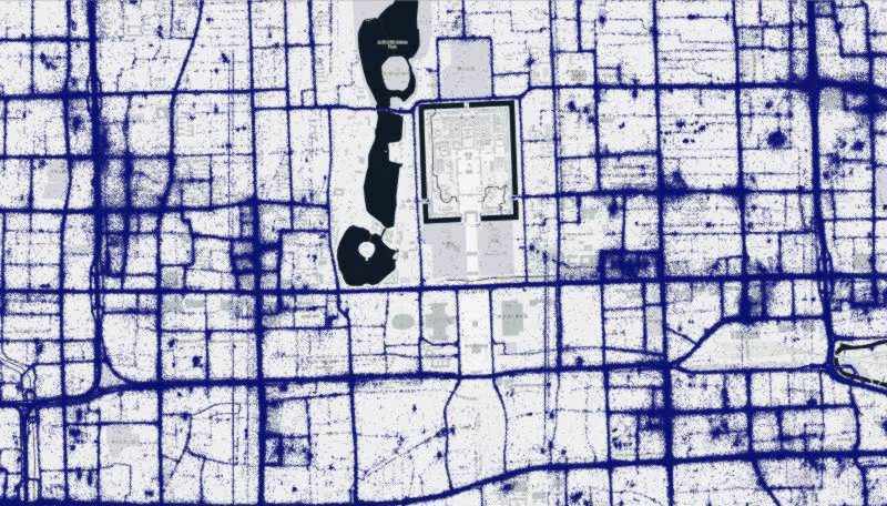
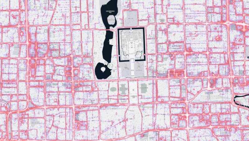
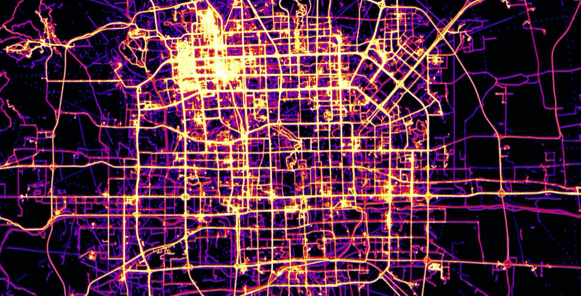
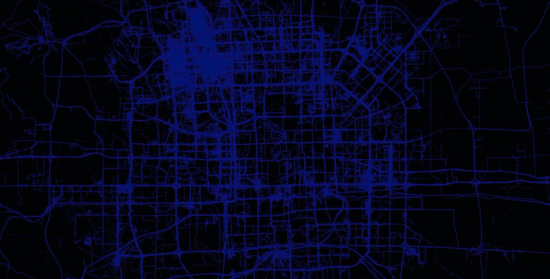
T-Drive
Microsoft research has made available a trajectory data set that contains the GPS coordinates of 10,357 taxis in Beijing, China and surrounding areas over a one week period. There are approximately 15 million points in this data set.
More information on this data set is available at: Microsoft Research T-drive page.
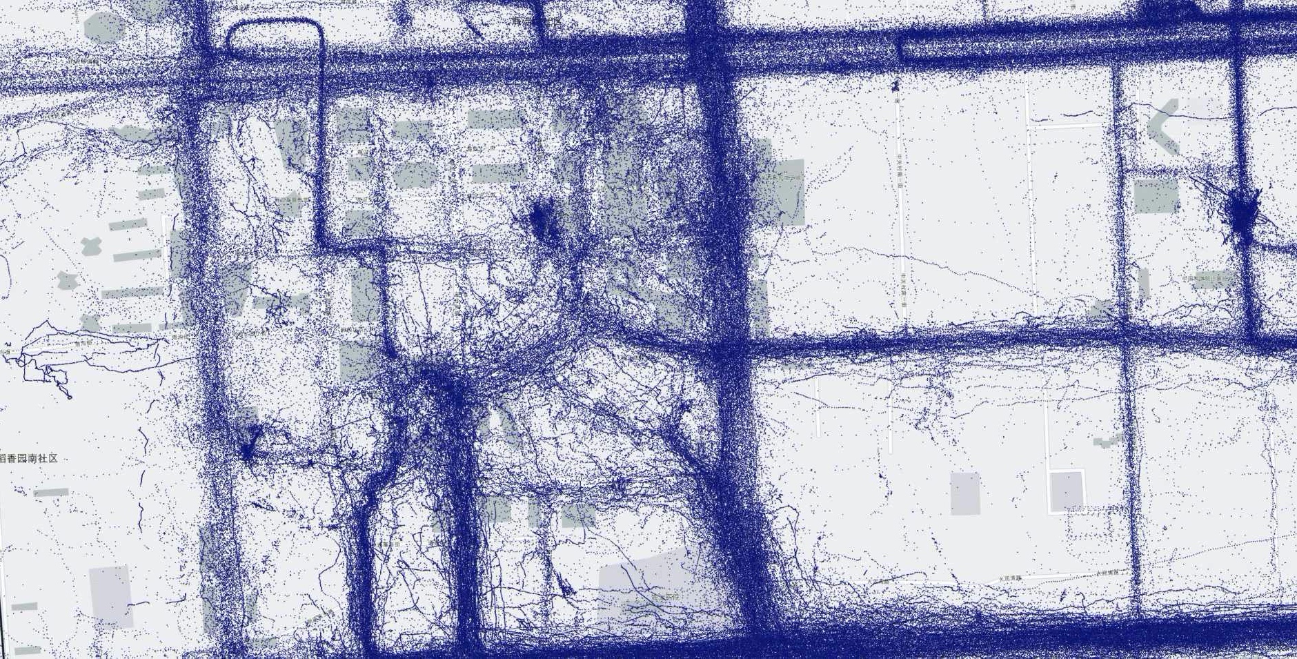
T-Drive at City Scale
Below are renderings of the t-drive data. They display the raw points along with the results of a GeoWave kernel density analytic. The data corresponds to Mapbox zoom level 12.