GeoWave Developer Guide
Introduction
Purpose of this Guide
This guide focuses on the development side of GeoWave. It also serves as a deep dive into some of the inner workings of GeoWave. The target audience for this guide are GeoWave developers and developers who wish to use GeoWave as part of another software package.
Assumptions
This guide assumes the following:
-
The reader is familiar with the basics of GeoWave discussed in the Overview.
-
The reader is familiar with the contents of the GeoWave User Guide.
-
GeoWave has already been installed and is available on the command-line. See the Installation Guide for help with the installation process.
Development Requirements
GeoWave development requires the following components:
-
Java Development Kit (JDK) (>= 1.8)
Requires JDK v1.8 or greater
Download from the Java downloads site. The OracleJDK is the most thoroughly tested but there are no known issues with OpenJDK.
-
Reference online material at Git SCM Site.
For a complete reference guide for installing and using Git, please reference chapters in the online Pro Git book.
-
Requires a version of Maven >= 3.2.1
For a reference guide for getting started with Maven, please reference the online Maven Getting Started Guide.
Development Setup
Retrieving the Code
Users have two options for retrieving the GeoWave source code: either by cloning the repository or by directly downloading the code repository as a ZIP archive.
Cloning the GeoWave Git Repository
The GeoWave code source can be cloned using the Git command-line interface. Using a Git clone allows the developer to easily compare different revisions of the codebase, as well as to prepare changes for a pull request.
| For developers who wish to make contributions to the GeoWave project, it is recommended that a fork of the main GeoWave repository be created. By submitting code contributions to a fork of GeoWave, pull requests can be submitted to the main repository. See the GitHub Forking documentation for more details. |
-
Navigate to the system directory where the GeoWave project code is to be located. The clone process will copy all of the repository’s contents to a directory called
geowave, it is therefore important to make sure that a directory calledgeowavedoes not already exist at the desired location. -
Clone the git repository by running the command:
$ git clone https://github.com/locationtech/geowave.gitIf you do not need the complete history, and want to speed up the clone, you can limit the depth of the checkout process by appending
-depth 1to the clone command above.The clone process can take several minutes and should produce output similar to the following:
Cloning into 'geowave'...
remote: Counting objects: 1311924, done.
remote: Compressing objects: 100% (196/196), done.
remote: Total 1311924 (delta 68), reused 0 (delta 0), pack-reused 1311657
Receiving objects: 100% (1311924/1311924), 784.52 MiB | 6.18 MiB/s, done.
Resolving deltas: 100% (1159959/1159959), done.
-
Confirm that the GeoWave contents were properly downloaded by examining the contents of the
geowavedirectory. The contents of the directory should be identical to the listings in the GeoWave GitHub repository.
Downloading the Code as ZIP Archive
This option is for users who do not intend to contribute to the GeoWave project source, but still would like to build or explore the source code. This is by far the simplest and most direct way to access the code.
To download a read-only version of the code repository:
-
Open a web browser and navigate to the GeoWave GitHub repository where the different projects and latest changes can be viewed.
-
If interested in a particular branch, select the branch of choice. Otherwise, leave on the default master branch for the latest tested changes.
-
Locate the green “Clone or download” button near the top right of the file navigation section.
-
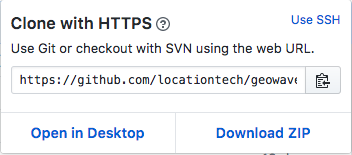
Expand the “Clone or download” pane by clicking on the green button labeled "Clone or download".
-
Download the code by clicking on the “Download ZIP” button. Depending on browser settings, the code will either download automatically to the user account’s downloads directory or a prompt will ask for the download destination. If the ZIP file is automatically downloaded to the downloads directory, manually move the ZIP file to the intended destination directory.
-
Navigate to the system directory where the ZIP file is located and unzip the contents.
Eclipse IDE Setup
The recommended Integrated Development Environment (IDE) for GeoWave is Eclipse. This section will walk you through importing the GeoWave Maven projects into the Eclipse IDE.
|
Setup and configuration of IDEs other than Eclipse are outside the scope of this document. If you do not wish to use Eclipse, there are likely guides available that discuss importing Maven projects into the IDE of your choice. |
Using the Eclipse Maven M2Eclipse plugin, we can import Maven projects into Eclipse. When importing Maven projects, Eclipse will automatically resolve and download dependencies listed in the pom.xml file for each project.
|
If a project’s |
-
Import the Maven GeoWave projects into the Eclipse workspace.
-
Within Eclipse, select File → Import.
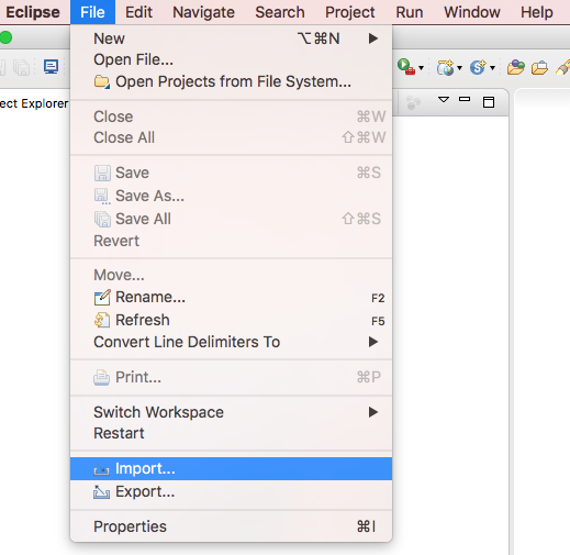 Figure 3. Eclipse File Import Menu
 -
From the "Import" window, select the option under "Maven" for "Existing Maven Projects" and select the "Next" button.
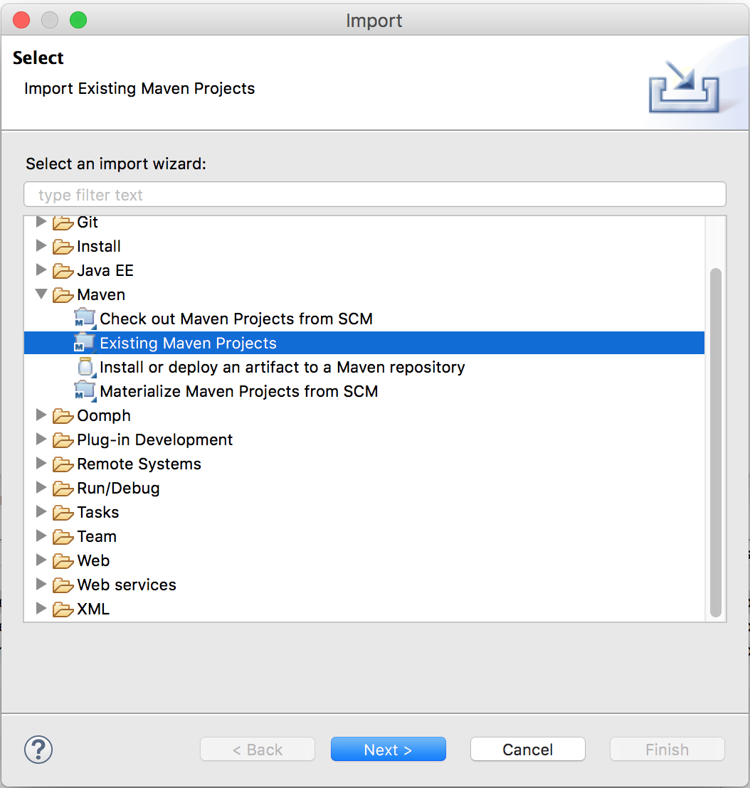 Figure 4. Existing Maven Projects Wizard
 -
From the "Import Maven Projects" window, select the “Browse” button and navigate to the root directory where the GeoWave source is located on the file system. Once found, select the geowave directory and select the "Open" button.
-
Within the "Import Maven Projects" window, the “Projects” pane should now be populated with all of the GeoWave projects. Select the "Finish" button to exit.
-
Upon returning to the workspace in Eclipse, the Project Explorer pane should now be populated with all of the GeoWave projects.
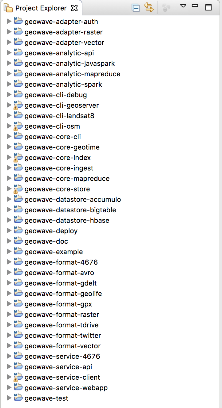 Figure 5. Eclipse Workspace
-
|
If Eclipse produces |
Clean Up and Formatter Templates
The GeoWave repository includes clean up and formatter templates that can be used by Eclipse to clean and format code according to GeoWave standards when those operations are performed in the IDE.
-
Within Eclipse, open the Eclipse Preferences window. (Eclipse → Preferences… on Mac, Window → Preferences on Windows and Linux).
-
Import clean up template:
-
Navigate to the Java → Code Style → Clean Up.
-
Press the "Import…" button.
-
Navigate to the
dev-resources/src/main/resources/eclipsedirectory from the GeoWave source, selecteclipse-cleanup.xml, and press the "Open" button. -
Press the "Apply" button.
-
-
Import formatter template:
-
Navigate to the Java → Code Style → Formatter.
-
Press the "Import…" button.
-
Navigate to the
dev-resources/src/main/resources/eclipsedirectory from the GeoWave source, selecteclipse-formatter.xml, and press the "Open" button. -
Press the "Apply and Close" button.
-
Now when Source → Clean Up… or Source → Format are used, they will be done in a manner consistent with the rest of the GeoWave source code.
Debugging
One of the simplest ways to debug GeoWave source code and analyze system interactions is to create a debug configuration and step through the integration test suite.
-
Within Eclipse open the Debug Configurations window (Run → Debug Configurations…).
-
Right-click on "JUnit" in the configuration type list on the left-hand side of the window and select "New Configuration".
-
Give the configuration a name, and ensure that
geowave-testis set in the "Project" field. -
Set the "Test Class" field to
org.locationtech.geowave.test.GeoWaveITSuite(or any other test class that is preferred). -
Navigate to the arguments tab and set values for the "VM arguments" field. Example:
-ea -DtestStoreType=ROCKSDB -DenableServerSideLibrary=falsewill run the test suite with RocksDB as the data store. Note: TheDenableServerSideLibraryoption technically only applies to Accumulo and HBase currently and is false by default. -
Click the "Apply" button to save the changes and then "Debug" to start the actual process.
The integration test suite allocates some resources on the local file system. If the suite is terminated or canceled before it finishes, it is possible that some of these resources may not be fully cleaned up by the test runner. This may cause issues or errors in subsequent runs of the suite. To resolve this issue, delete the temp folder and the <DataStoreName>_temp folder where <DataStoreName> is the name of the data store used by the current debug configuration. Both of these folders will exist under the target directory of the geowave-test project.
Building the Source
Building GeoWave
To build the project source, navigate to the root directory of the GeoWave project using a command-line tool and execute the following maven command:
$ mvn clean install (1) (2)| 1 | You can speed up the build by skipping unit tests and bug checks by adding -Dfindbugs.skip -Dspotbugs.skip -DskipTests |
| 2 | You can prevent GDAL-related tests from running by setting an environment variable called GDAL_DISABLED to true: export GDAL_DISABLED=true |
After executing the command, Maven will search for all of the projects that need to be built and begin the build process. The initial output of the command should look something like the following:
[INFO] Scanning for projects...
[INFO] ------------------------------------------------------------------------
[INFO] Reactor Build Order:
[INFO]
[INFO] GeoWave Parent POM
[INFO] GeoWave Core Parent POM
[INFO] GeoWave CLI
[INFO] GeoWave Index
[INFO] GeoWave Store
.
.
.
The build process can take several minutes, but once this is completed, the compiled artifacts for each project will be installed to your local Maven repository. They will also be available in each project’s target directory.
Running Integration Tests
By default, integration tests are not run as part of the normal build process. This is because integration tests can be run for a multitude of key/value store backends, and tests for a single backend can take a significant amount of time to complete. Usually these integration tests are run through GitHub Actions, but it can be useful to run them locally when working on code that could potentially impact one of the tests.
Integration tests are all written in the geowave-tests project and are run using a series of Maven profiles. The following table shows the various profiles available along with a description of the tests that are run:
| Maven Profile | Description |
|---|---|
accumulo-it-client |
Run integration tests on Accumulo with server-side libraries disabled |
accumulo-it-server |
Run integration tests on Accumulo with server-side libraries enabled |
accumulo-it-all |
Run integration tests on Accumulo with server-side libraries enabled and disabled |
bigtable-it |
Run integration tests on Bigtable |
cassandra-it |
Run integration tests on Cassandra |
dynamodb-it |
Run integration tests on DynamoDB |
hbase-it-client |
Run integration tests on HBase with server-side libraries disabled |
hbase-it-server |
Run integration tests on HBase with server-side libraries enabled |
hbase-it-all |
Run integration tests on HBase with server-side libraries enabled and disabled |
kudu-it |
Run integration tests on Kudu |
redis-it |
Run integration tests on Redis |
rocksdb-it |
Run integration tests on RocksDB |
secondary-index-it |
Run integration tests with secondary indexing enabled, this profile can be used with any of the previous profiles |
In order to use one of these profiles to run integration tests, use the same command that was used to build the source, but add the appropriate profile to the end. For example, if you wanted to run integration tests for RocksDB, the command would look like the following:
$ mvn clean install -Procksdb-itIf you have already built GeoWave, you can skip straight to the integration tests:
$ mvn clean install -rf :geowave-test -Procksdb-itBuilding Python Bindings
The Python bindings for GeoWave (pygw) use a different build process than the Java component. The Python source code for pygw can be found in the python/src/main/python directory. In order to install pygw from source, you will need Python 3 (up to Python 3.7) and Virtualenv.
Building the Wheel
Navigate to Python source directory python/src/main/python in your command-line tool and perform the following steps.
Create the virtual environment:
$ virtualenv -p python3.7 venvActivate the environment:
$ source venv/bin/activateInstall requirements in the activated python virtual environment:
$ pip install -r requirements.txt
Install necessary build tools:
$ pip install --upgrade pip wheel setuptools twineBuild the wheel:
$ python setup.py bdist_wheel --python-tag=py3 sdistInstalling the Wheel
After performing the steps in the build step, a .whl file should be written to the dist directory. To install it, simply perform the pip install command on that file:
$ pip install dist/pygw-*.whl
If you have multiple wheel builds in the dist directory, use the full filename of the .whl you wish to install.
|
Running Tests
In order to run tests for pygw, a GeoWave Py4J Java Gateway needs to be running. GeoWave offers a simple CLI command to run a gateway. In a separate window, execute the following command:
$ geowave util python rungateway
If GeoWave was installed using the standalone installer, this command is only available if the Python Tools component was included.
|
While this gateway is running, execute the following command to run the tests:
$ python -m pytestBuilding Docs
GeoWave documentation consists of several different parts, the main documentation, which includes this guide, the Javadocs, and the Python bindings documentation.
GeoWave Documentation
GeoWave documentation is primarily written with Asciidoctor and can be built using a single Maven command from the GeoWave root directory:
$ mvn -P html -pl docs install -DskipTests -Dspotbugs.skipThis command compiles all documentation as HTML and outputs it to the target/site directory.
PDF output is also supported by replacing -P html in the above command with -P pdf.
|
Javadocs
Javadocs for all projects can be built using the following command:
$ mvn -q javadoc:aggregate -DskipTests -Dspotbugs.skipThis command will output all of the Javadocs to the target/site/apidocs directory.
Python Bindings Documentation
They GeoWave Python bindings been documented using Python docstrings. In order to generate this documentation, a Python environment should be set up and the GeoWave Py4J Java Gateway should be running, see Build Python Bindings for help with this. Once the environment is activated an the gateway is running, execute the following command from the python/src/main/python directory to generate the documentation:
$ pdoc --html pygwThis will generate the Python API documentation in the python/src/main/python/html/pygw directory.
Docker Build Process
We have support for building both the GeoWave JAR artifacts and RPMs from Docker containers. This capability is useful for a number of different situations:
-
Jenkins build workers can run Docker on a variety of host-operating systems and build for others
-
Anyone running Docker will be able to duplicate our build and packaging environments
-
Will allow us to build on existing container clusters instead of single purpose build VMs
If building artifacts using Docker containers interests you, check out the README in deploy/packaging/docker.
Packaging GeoWave Builds
GeoWave can be packaged in several different ways. Prior to packaging GeoWave, make sure that the build process has completed.
GeoWave CLI Tools
GeoWave artifacts can be packaged into a single JAR that can be used to execute CLI commands by running the following Maven command from the GeoWave root directory:
$ mvn package -P geowave-tools-singlejar -Dfindbugs.skip -Dspotbugs.skip -DskipTestsAfter the packaging process is complete, the resulting JAR will be available in the deploy/target directory with a name like geowave-deploy-<version>-geoserver.jar. To use this jar for CLI commands you can execute it using the following java command:
$ java -cp java -cp <geowave_home>/deploy/target/geowave-deploy-2.0.1-tools.jar org.locationtech.geowave.core.cli.GeoWaveMain <command> <options>
Replace <geowave_home> with the GeoWave home directory, or use an environment variable.
|
As you can see, using GeoWave in this way can be fairly cumbersome. To make things easier, this command can be wrapped up in an alias.
$ alias geowave="java -cp $GEOWAVE_HOME/deploy/target/geowave-deploy-2.0.1-tools.jar org.locationtech.geowave.core.cli.GeoWaveMain"$ doskey geowave=java -cp %GEOWAVE_HOME%/deploy/target/geowave-deploy-2.0.1-tools.jar org.locationtech.geowave.core.cli.GeoWaveMain $*After the alias has been created, you will be able to use the GeoWave CLI with the geowave command. For a full list of these commands, please see the GeoWave CLI Appendix.
GeoServer Plugin
GeoWave artifacts can be packaged into a single JAR to be used in a GeoServer installation by running the following Maven command from the GeoWave root directory:
$ mvn package -P geotools-container-singlejar -Dfindbugs.skip -Dspotbugs.skip -DskipTestsAfter the packaging process is complete, the resulting JAR will be available in the deploy/target directory with a name like geowave-deploy-<version>-geoserver.jar. To use this jar with a GeoServer installation, simply copy it to the WEB-INF/lib directory of GeoServer’s installation and restart the web service that GeoServer is running on.
Accumulo JAR
GeoWave artifacts can be packaged into a JAR to be used by Accumulo for server-side operations by running the following Maven command from the GeoWave root directory:
$ mvn package -P accumulo-container-singlejar -Dfindbugs.skip -Dspotbugs.skip -DskipTestsAfter the packaging process is complete, the resulting JAR will be available in the deploy/target directory with a name like geowave-deploy-<version>-accumulo.jar. See Accumulo Configuration in the User Guide for more information about using this jar.
HBase Coprocessor JAR
GeoWave artifacts can be packaged into a coprocessor JAR for HBase server-side operations by running the following Maven command from the GeoWave root directory:
$ mvn package -P hbase-container-singlejar -Dfindbugs.skip -Dspotbugs.skip -DskipTestsAfter the packaging process is complete, the resulting JAR will be available in the deploy/target directory with a name like geowave-deploy-<version>-hbase.jar. In order to use this jar, copy it to an HDFS location that is accessible to HBase. When configuring the GeoWave HBase data store (either through the GeoServer plugin or the CLI), set the coprocessorJar option to the HDFS location of the jar.
Standalone Installers
Standalone installers for Linux, Mac, and Windows can be built using Install4J.
| Installers are built using Install4J, which requires an active license to use. This section of the guide assumes that Install4J has been installed on the system and has a valid license. |
Several things need to be done in order to successfully build the standalone installers, each of which are outlined below.
Build GeoWave Artifacts
The installers require all of the GeoWave artifacts to be built prior to packaging. See Building GeoWave for help with building the artifacts.
Build GeoWave Documentation
The installers provide an option to the user to install documentation, because of this, all documentation should be built prior to packaging the installers. SeeBuilding Documentation for help with building all of the documentation.
After building the Python documentation, move the python/src/main/python/html/pygw directory to the target/site directory and rename it to pydocs. This will prevent broken links in the generated documentation.
|
| This step can be skipped, but the the documentation directory of the GeoWave installation will be empty. This can save some time if the installer is only intended to be used for testing purposes. |
Package Installer Plugins
The installers provide several ways for users to customize their installation of GeoWave. This is handled by packaging GeoWave extensions and optional components as installer plugins. All installer plugins in the GeoWave codebase can be packaged using the following Maven command:
$ mvn package -P build-installer-plugin -DskipTests -Dfindbugs.skip -Dspotbugs.skipThis will package all of the installer plugins and put them into directories expected by the Install4J build process.
Build Installers
Once all of the above steps have been completed, the GeoWave standalone installers can be built using the following Maven command:
$ mvn package -pl deploy -P build-installer-main -Dinstall4j.home=$INSTALL4J_HOME -DskipTests -Dfindbugs.skip -Dspotbugs.skipThis command expects an environment variable $INSTALL4J_HOME that points to the root directory of the Install4J installation. Once the command is complete, standalone installers for Linux, Mac, and Windows will be available in the deploy/target/install4j-output directory.
How to Contribute
GeoWave is an open source project and we welcome contributions from the community.
Pull Requests
Pull requests must be done though a forked repository.
To create a new fork, just click the the "Fork" button at the top of the GeoWave GitHub page. You can now submit pull requests from your working branch on your fork directly to the master branch on the locationtech repository.
GeoWave uses a Maven plugin formatter to keep all of our code standardized. You should run a Maven install immediately prior to committing and pushing changes.
Prior to submitting a pull request, please squash down your commits into one. This will help keep our commit history clean and will cut down on "in progress commits" that don’t relay any helpful information in the future.
All contributors must sign the Eclipse Contributor Agreement and sign off all commits by using the --signoff option of the commit command.
All pull request contributions to this project will be released under the Apache 2.0 license.
Software source code previously released under an open source license and then modified by NGA staff is considered a "joint work" (see 17 USC 101); it is partially copyrighted, partially public domain, and as a whole is protected by the copyrights of the non-government authors and must be released according to the terms of the original open source license.
Architecture
Overview

The core of the GeoWave architecture concept is getting data in (Ingest), and pulling data out (Query). This is accomplished by using data adapters and indices. As discussed in the GeoWave Overview, data adapters describe the available fields in a data type and are used to transform data from the base type into a format that is optimized for GeoWave. An index is used to determine the organization and storage of the converted data so that it can be efficiently queried. There are two types of data persisted in the system: indexed data and metadata. Indexed data is the data (such as vector attributes and geometries) that has been converted to the GeoWave format by an adapter and stored using the index. Metadata contains all of the information about the state of the data store, such as the adapters, indices, and any statistics that have been created for a type. The intent is to store all of the information needed for data discovery and retrieval in the database. This means that an existing data store isn’t tied to a bit of configuration on a particular external server or client but instead is “self-describing.”
Key Structure
The following diagram describes the default structure of indexed data in a GeoWave data store.

These structures are described by two interfaces: GeoWaveKey and GeoWaveValue. It is up to the data store implementation to determine how to use these structures to ultimately store GeoWave data, so the final structure may vary between implementations.
GeoWave Key
-
Partition Key: This key is derived from the partition strategy used by the index. By default, no partitioning strategy is used and this portion of the key will be empty. GeoWave also provides round robin and hash-based partitioning strategies.
-
Sort Key: This key is derived from the index strategy and is the main factor in determining the sort order of entries in the key/value store. In most cases this will be a result of the SFC implementation used by the index.
-
Internal Adapter ID: This is a short which represents the adapter that the data belongs to. This internal ID is used instead of the full adapter name to save space. A mapping between internal adapter ID and adapter exists in the metadata tables of the GeoWave data store. This is encoded with variable length encoding.
-
Data ID: An identifier for the data represented by this row. We do not impose a requirement that Data IDs are globally unique but they should be unique for the adapter. Therefore, the pairing of Internal Adapter ID and Data ID define a unique identifier for a data element. An example of a data ID for vector data would be the feature ID.
-
Data ID Length: The length, in bytes, of the Data ID, encoded with variable length encoding.
-
Number of Duplicates: The number of duplicates is stored to inform the de-duplication filter whether this element needs to be temporarily stored in order to ensure no duplicates are sent to the caller.
GeoWave Value
-
Field Mask: This mask represents the set of fields from the data type that are visible in this row.
-
Visibility: The visibility expression used by this row of data. It is possible for a single data entry to have different visibility expressions on different attributes. In this case, the entry will be split into multiple rows, with each row having a different Visibility and a Field Mask that indicates which fields are represented by that visibility expression. The visibility of an entry is determined by passing the entry to a
VisibilityHandler. The handler that is used is generally set when a type is created, but can be overridden by passing a different handler when creating the writer. -
Value: The extended data of the entry.
Data Stores
GeoWave data stores are made up of several different components that each manage different aspects of the system, such as an adapter store, index store, statistics store, etc. Most of the time, directly using these components should not be necessary as most GeoWave tasks can be accomplished through the use of the DataStore interface.
Programmatically, data stores are accessed by using a StoreFactoryOptions implementation for the appropriate key/value store to configure a connection to that store. Once configured with all of the necessary options, the DataStoreFactory can be used to directly create a DataStore instance.
An instance of DataStorePluginOptions can be also be created from the StoreFactoryOptions if direct access to other parts of the data store is needed.
For an example of accessing a data store through the programmatic API, see the Creating Data Stores example.
Indices
The way that GeoWave stores data in a way that makes it efficient to query is through the use of Indices. As mentioned in the overview, indices use a given set of dimensions to determine the order in which the data is stored. Indices are composed of two components: a common index model, and an index strategy.
Common Index Model
The common index model defines the set numeric dimensions expected by an index. For example, a spatial-temporal index might have 3 dimensions defined by the model: latitude, longitude, and time. In order for data to be added to that index, it must supply all of the dimensions required by the model. The data adapter is responsible for associating attributes from the raw data type with the dimensions of the common index model.
Index Strategies
An index strategy is what dictates how the dimensioned data from the index model are used to structure the data in the data store. When data is added to GeoWave, an index strategy is applied to determine the Partition Key and Sort Key of the data. Determining which index strategy to use is dependent on the nature of the data and the types of queries that will be performed.
While most GeoWave index strategies implement the IndexStrategy interface, there are currently two main types of index strategies: sorted index strategies, and partition index strategies. Sorted index strategies use one or more dimensions from the index model to sort the data in a predictable way. Partition index strategies can be used to split data that would usually reside next to each other into separate partitions in order to reduce hotspotting during querying.
IndexStrategy Hierarchy
The diagram below outlines the hierarchy of the various index strategies currently available within GeoWave.

Most of GeoWave’s index strategies are derived from NumericIndexStrategy, which is the only SortedIndexStrategy implementation included with GeoWave. The NumericIndexStrategy also implements the PartitionIndexStrategy interface so that any derived strategy can define its own partitioning methods. Any numeric index strategy can also be partitioned using one of the built-in PartitionIndexStrategy implementations by using a CompoundIndexStrategy which wraps a NumericIndexStrategy and a PartitionIndexStrategy into a single strategy. The HierarchicalNumericIndexStrategy implementations are where most of the built-in spatial and spatial-temporal indexing is done. See the Theory section for more information about how GeoWave hierarchical indexing works.
There are two built-in PartitionIndexStrategy implementations. The round robin partition index strategy evenly distributes data to one of N partitions in a round robin fashion, i.e. every successive row goes to the next successive partition until the last partition is reached, at which point the next row will go to the first partition and the process repeats. The hash partition index strategy assigns each row a partition based on the hash of dimensional data. This should also result in a fairly even row distribution. Unlike the round robin strategy, the hash strategy is deterministic. This means that the partition that a row will go to will not change based on the order of the data.
If there is no suitable index strategy implementation for a given use case, one can be developed using any of the built-in strategies as a reference.
Custom Indices
If more direct control of an index is required, a custom index can be created by implementing the CustomIndexStrategy interface. This interface is the most straightforward mechanism to add custom indexing of any arbitrary logic to a GeoWave data store. It is made up of two functions that tell GeoWave how to index an entry on ingest and how to query the index based on a custom constraints type. The interface has two generics that should be supplied with the implementation. The first is the entry type, such as SimpleFeature, GridCoverage, etc. The second is the constraints type, which can be anything, but should implement the Persistable interface so that it can work outside of client code. The constraints type is a class that is used by the CustomIndexStrategy implementation to generate a set of query ranges for the index based on some arbitrary constraint.
Once a CustomIndexStrategy implementation has been created, an index can be created by instantiating a CustomIndex object with the custom index strategy and an index name. An example implementation of a custom index is available in the geowave-example project.
Custom indices are different from other GeoWave indices in that they do not conform to the marriage of a common index model and an index strategy. Because custom indices provide direct control over the indexing of data, it is up to the developer to decide how the indexing should work. Because of this, it is important to note that the CustomIndexStrategy interface has no relation to the IndexStrategy interface used by the core GeoWave indices.
|
Secondary Indexing
When secondary indexing is enabled on a data store, all data is written to a DATA_ID index in which the key is a unique data ID. Indices on that data store will then use this data ID as the value instead of the encoded data. This can be useful to avoid excessive duplication of encoded data in cases where there are many indices on the same dataset. The drawback for secondary indexing is that when data needs to be decoded, GeoWave has to do a second lookup to pull the data out of the DATA_ID index.
Adapters
In order to store geometry, attributes, and other information, input data must be converted to a format that is optimized for data discovery. GeoWave provides a DataTypeAdapter interface that handles this conversion process. Implementations that support GeoTools simple feature types as well as raster data are included. When a data adapter is used to ingest data, the adapter and its parameters are persisted as metadata in the GeoWave data store. When the type is queried, the adapter is loaded dynamically in order to translate the GeoWave data back into its native form.
Feature Serialization

GeoWave allows developers to create their own data adapters. Adapters not only dictate how the data is serialized and deserialized, but also which attributes should be used for a given index. GeoWave’s goal is to minimize the code and make the querying logic as simple as possible. This conflicts with the desire to allow maximum flexibility with arbitrary data adapters. To solve this, data from an adapter is split between common index data and extended data. Common index data are non-null numeric fields that are used by the index. They can also be used in server-side filtering during a query without having to decode the entire entry. Extended data is all of the remaining data needed to convert the entry back into its native form. Any filtering that needs to be done on this extended data would require that the entry be decoded back into its native form. This would be done client-side and would have a significant impact on query performance.
Common Index Data
Common index data are the fields used by the index to determine how the data should be organized. The adapter determines these fields from the common index model that is provided by the index when data is encoded. Common index data fields will typically be geometry coordinates and optionally time, but could be any set of numeric values. These fields are used for fine-grained filtering when performing a query. Common index data cannot be null.
Extended Data
Extended data is all of the remaining data needed to convert the entry back into its native form. Any filtering that needs to be done on this extended data would require that the entry be decoded back into its native form. This would be done client-side and would have a significant impact on query performance. The data adapter must provide methods to serialize and deserialize these items in the form of field readers and field writers. As this data is only deserialized client-side, the readers and writers do not need to be present on the server-side classpath.
Field Writers/Readers
Field readers and writers are used by data adapters to tell GeoWave how to serialize and deserialize data of a given type. GeoWave provides a basic implementation for the following attribute types in both singular and array form:
Boolean |
Byte |
Short |
Float |
Double |
BigDecimal |
Integer |
Long |
BigInteger |
String |
Geometry |
Date |
Calendar |
Field readers must implement the FieldReader interface, and field writers must implement the FieldWriter interface.
Internal Adapter ID
Most public interfaces and tools reference adapters by their name, however, it would be redundant to include this full name in every row of the database. GeoWave reduces this memory impact by mapping each adapter to an 2 byte (short) internal adapter ID. This mapping is stored in a metadata table and can be looked up using the InternalAdapterStore.
Statistics
Overview
GeoWave statistics are stored as metadata and can be queried for aggregated information about a particular data type, field, or index. Statistics retain the same visibility constraints as the data they are associated with. For example, let’s say there is an data type that has several rows with a visibility expression of A&B, and several more rows with a visibility expression of A&C. If there was count statistic on this data, then there would be two rows in the statistics table, one for the number of rows with the A&B visibility, and another for the number of rows with the A&C visibility.
Statistic Types
There are three different types of statistics, each of which extend from a different base statistic class.
Index Statistics
Index statistics are statistics that are tracked for all rows in a given GeoWave index. They derive from IndexStatistic and include an option that specifies the index name that the statistic belongs to. These statistics are usually quite broad as they cannot make assumptions about the data types that are included in the index. Some examples of index statistics are row range histograms, index metadata, and duplicate entry counts. Many of these statistics are binned using the DataTypeBinningStrategy so that information about any of these statistics can be queried on a per-data-type basis if needed.
Data Type Statistics
Data type statistics are statistics that are tracked for all rows for a given data type. They derive from DataTypeStatistic and include an option that specifies the data type name that the statistic belongs to. The main example of this type is the count statistic, which simply counts the number of entries in a given data type.
Field Statistics
Field statistics are statistics that are tracked for a given field of a single data type. They derive from FieldStatistic and include options for both the data type name and the field name to use. Each field statistic includes a method that determines whether or not it is compatible with the java class of a given field. For example, a numeric mean statistic only supports fields that derive from Number so that it can calculate the mean value of the field over the entire data set. This compatibility check allows statistics to be implemented and re-used across all data types that use the same field class.
Binning Strategies
Sometimes it is desirable to split up a statistic into several bins using some arbitrary method. Each bin is identified by a unique byte array and contains its own statistic value for all rows that fall into it. GeoWave includes a few binning strategies that cover a majority of simple use cases.
-
DataTypeBinningStrategy: The
DataTypeBinningStrategyis a binning strategy that can be used on index statistics to create a separate bin for each data type in the index. -
PartitionBinningStrategy: The
PartitionBinningStrategyis a binning strategy that is generally only used by internal statistics that creates a separate bin for each partition that the data resides on. -
FieldValueBinningStrategy: The
FieldValueBinningStrategyis a binning strategy that can be used on any statistic to create a separate bin for each unique value of a given field or set of fields. For example, if a data type had aCountryCodefield, this binning strategy could be used on aCOUNTstatistic to count the number of entries for each uniqueCountryCodevalue. If a data type had bothShapeandColorfields, this strategy could be used to combine both to count the number of entries for eachShape/Colorcombination. -
NumericRangeFieldValueBinningStrategy: The
NumericRangeFieldValueBinningStrategyis a binning strategy that can be used on any statistic to create a separate bin for defined ranges of a given numeric field or set of fields. For example, if a data type had a numericAnglefield, this binning strategy could be used on aCOUNTstatistic to count the number of entries in each angle range defined by a user-supplied interval. Like theFieldValueBinningStrategy, this strategy can be used with multiple numeric fields. -
TimeRangeFieldValueBinningStrategy: The
TimeRangeFieldValueBinningStrategyis a binning strategy that can be used on any statistic to create a separate bin for defined ranges of a given temporal field or set of fields. For example, if a data type had a time field calledStartTime, this binning strategy could be used on aCOUNTstatistic to count the number of entries in each year, month, week, day, hour, or minute defined by theStartTimeof the entry. Like theFieldValueBinningStrategy, this strategy can be used with multiple temporal fields. -
CompositeBinningStrategy: The
CompositeBinningStrategyallows two binning strategies to be combined. This strategy can be used when a single binning strategy is not sufficient to split the statistic in the desired way.
In order to provide as much flexibility as possible to developers, the StatisticBinningStrategy interface has been made available so that new binning strategies can be added as the need arises. This is described in more detail below.
Table Structure
Statistics are composed of two different types of objects that are stored within the GeoWave metadata tables: statistics and the statistic values.
The statistic table contains all of the tracked statistics for the data store. Each row of this table describes one statistic and contains all of the information needed to properly calculate the statistic as data is ingested and deleted.
The following diagram describes the default structure of a statistic in a GeoWave data store.

-
Unique ID: A unique identifier for the statistic within a given statistic group. The unique identifier is composed of the statistic type, a field name (for field statistics), and a tag. Different statistic groups can have a statistic with the same unique identifier. For example, two different data types could have a
COUNTstatistic with a tag ofinternalbecause they are in different statistic groups. -
Group ID: The group that the statistic belongs to. This identifier is composed of a type specifier and a group, which can vary based on the type of statistic. The type specifier is a single byte that indicates if the statistic is an index statistic, a data type statistic, or a field statistic. The group is the index or type name that the statistic is associated with.
-
Serialized Statistic: All information needed to calculate the statistic when data is ingested or deleted. This includes any binning strategies or other options used by the statistic.
The values of these statistics are stored separately as GeoWave metadata with a similar structure.

-
Statistic Unique ID: The unique ID of the underlying statistic.
-
Bin: The bin for the statistic, if the statistic uses a binning strategy.
-
Statistic Group ID: The group ID of the underlying statistic.
-
Visibility: The visibility expression represented by this statistic value. It is possible for a dataset to have different visibility expressions on different rows. In this case, there will be a separate statistic value for each unique visibility expression.
-
Statistic Value: The serialized value for this bin.
Getting Statistic Values
There are two primary ways to get the value of a given statistic. The first and easiest way is to use the Statistic object itself as a parameter to getStatisticValue or getBinnedStatisticValues on the DataStore interface. If the statistic uses a binning strategy, a set of bin constraints can also be supplied to filter down the bins that are returned by the query. Each binning strategy supports different types of constraints, which can be discovered through the supportedConstraintClasses method. These constraint classes can be converted into bin constraints by passing them to the constraints method on the binning strategy. For example, TimeRangeFieldValueBinningStrategy supports Interval as a constraint class. All bins within a given time interval could be queried by passing the result of constraints(interval) to the getStatisticValue method on the DataStore. These methods do not take visibility of rows into account and will get the values for all visibilities by default.
The second way statistic values can be retrieved is to query the statistic by using a StatisticQueryBuilder. A query builder of the appropriate type can be obtained by calling one of the newBuilder static methods on StatisticQueryBuilder with the StatisticType to query. Once all of the query parameters and optional constraints have been set and the query is built, the resulting StatisticQuery object can then be passed to the queryStatistics or aggregateStatistics functions of the DataStore. Each of these functions performs the same query, but outputs different values. The queryStatistics function will return one StatisticValue instance for every bin for each statistic that matched the query parameters, while the aggregateStatistics function will merge all of those values down to a single StatisticValue instance. A statistic query allows you to provide authorizations if the result should be filtered by visibility.
|
When querying statistics with varying visibilities, GeoWave will merge all statistics that match the provided authorizations. Using the following example, providing no authorizations would return a count of 0, providing 
Figure 12. Statistics Merge
|
Implementing New Statistics and Binning Strategies
New statistics can be implemented by extending the appropriate statistic type (IndexStatistic, DataTypeStatistic, or FieldStatistic) and implementing a corresponding StatisticValue. It is recommended that a public static STATS_TYPE variable be made available to make the StatisticType of the statistic readily available to users.
New binning strategies can also be added by implementing the StatisticBinningStrategy interface. The binning strategy can use information from the DataTypeAdapter, the raw entry, and the GeoWaveRow(s) that the entry was serialized to in order to determine the bin that should be used. It is also recommended to provide some level of support for constraints that would be relevant to the binning strategy to make it easier for end users to constrain statistics queries.
All statistics and binning strategies are discovered by GeoWave using Service Provider Interfaces (SPI). In order to add new statistics and binning strategies, extend the StatisticsRegistrySPI and make sure the JAR containing both the registry and the statistic/statistic value classes are on the classpath when running GeoWave. For more information on using SPI, see the Oracle documentation.
An example that shows how to add a word count statistic is available in the GeoWave examples project.
Ingest
Overview
In addition to the raw data, the ingest process requires an adapter to translate the native data into a format that can be persisted into the data store, and an index to dictate how the ingested data should be organized. The following diagram shows an overview of the ingest process:

The logic within the ingest process immediately ensures that the index and data adapter are persisted as metadata within the index and adapter stores to support self-described data discovery. In-memory implementations of both of these stores are provided for cases when connections to third-party data stores (e.g., Accumulo, HBase) are undesirable in the ingest process, such as ingesting bulk data in a MapReduce job. Once the adapter and index have been persisted, each data entry gets processed by the adapter to encode the data to a format that’s optimized for GeoWave, and by the index to determine where the data should be stored.
| Certain circumstances will cause the same data to be written to the data store in multiple locations, e.g., polygons that cross the dateline or date ranges that cross binning boundaries such as December 31-January 1 when binning by year. To remedy this, deduplication is always performed as a client filter when querying the data. |
Once the GeoWaveKey and GeoWaveValue are created for an entry, they are combined into a GeoWaveRow and sent to the RowWriter implementation to be written to the data store.
The full list of GeoWave ingest commands can be found in the GeoWave CLI Documentation.
Ingest Plugins
Ingest plugins contain everything that is needed to convert raw data files into a format that is understood by a GeoWave data adapter. Ingest plugins hook into the ingest framework and are decoupled from the data store and index implementations.
Source Formats
Leveraging the GeoTools infrastructure, GeoWave supports ingesting any DataSource that GeoTools supports. Currently supported data types include:
-
arcgrid
-
arcsde
-
db2
-
raster formats
-
geotiff
-
grassraster
-
gtopo30
-
imageio-ext-gdal
-
imagemoasaic
-
imagepyramid
-
JP2K
-
-
Database “jdgc-ng” support
-
h2
-
mysql
-
oracle
-
postgis
-
spatialite
-
sqlserver
-
-
postgis
-
property file
-
shapefile
-
dfs
-
edigeo
-
geojson
-
wfs
For a current list of supported formats, refer to the GeoTools User Guide. Reference the version of GeoTools that GeoWave was built against (currently 20.0).
Adding New Plugins
For raw data input formats that aren’t supported by GeoWave directly, new ingest plugins can be written and installed to enable those unsupported formats to be ingested. The simplest way to create a new ingest plugin is to extend the MinimalSimpleFeatureIngestFormat and MinimalSimpleFeatureIngestPlugin classes. These classes ask a user to define a schema for their data as a SimpleFeatureType and read data from a URL as SimpleFeatures. With this information, GeoWave can handle the rest of the ingest process. Once registered via SPI, the custom format will be able to be used to ingest files of the custom format via the CLI or programmatically. An example implementation of a minimal ingest plugin is available in the geowave-example project.
Sometimes it becomes necessary to have more control over the ingest process, such as allowing features to be ingested from an optimized Avro format or via mapreduce. In this case there are additional options for implementing ingest plugins. For vector data, GeoWave expects plugins to convert the source data into GeoTools SimpleFeature objects. For raster data it expects GeoTools GridCoverage objects. Additionally, a data format can supply a translation from a file to any custom schema, which can then be used as an intermediate format to support distributed ingest. For example, all built-in vector ingest plugins derive from AbstractSimpleFeatureIngestPlugin which itself implements GeoWaveAvroFormatPlugin. This allows the data to be converted into an intermediate Avro format, which can then be ingested in a distributed fashion.
New vector ingest plugins should extend the AbstractSimpleFeatureIngestPlugin class. See the GeoToolsRasterDataStoreIngestPlugin for an example of a plugin that ingests raster data.
Any of our extensions/formats projects are good examples for supporting new formats that can be discovered at runtime, such as the GeoWaveAvroIngestPlugin, or any of the other existing ingest plugins, such as those listed in the extensions/formats directory.
New ingest formats are discovered using Service Provider Interface (SPI)-based injection. In order to install a new ingest format, implement IngestFormatPluginProviderSpi and make sure your JAR is on the classpath when running GeoWave. For more information on using SPI, see the Oracle documentation.
Query
A query in GeoWave is composed of a set of filters and index constraints. Index constraints are the portions of the query filter that affect the index dimensions. For example, the geometry from a spatial filter can be used as index constraints when querying a spatial index.
Overview

When a query is performed, GeoWave extracts index constraints from the provided query filter. These index constraints are then decomposed into a set of range queries according to the index strategy that is used by the index. See the Theory section for information about how ranges are decomposed for multi-dimensional data. These range queries represent the coarse grain filtering of the query.
The query filter is broken down into two types of filters: distributable and client. Distributable filters are filters that operate on the common index data while client filters are filters that operate on the extended data of the feature. Distributable filters are serialized and sent to the data store in order to filter the results of the range queries server-side. An example of a distributable filter is a geometry filter. The index constraints extracted from the geometry filter are generally loser than the actual geometry to simplify the number of range queries that need to be performed. Because of this, results from the range queries must pass through the actual geometry filter to remove any entries that do not match exactly.
All results that pass the distributable filters are then returned to the client which decodes each entry using the data adapter and discards any entries that do not pass the remaining client filters.
| Currently only HBase and Accumulo data stores support distributable filters. All other data store types will perform all filtering on the client. |
Query Builders
Queries are created in GeoWave through the use of query builders. These builders are used to set all the things needed to create a query, such as the type names, indices, authorizations, and query constraints. While the base QueryBuilder can be used as a general way to query data, GeoWave also provides an implementation of the query builder that is specific to vector queries with the VectorQueryBuilder. It also provides a query builder for vector aggregation queries with the VectorAggregationQueryBuilder. These vector query builders provide a constraints factory that has additional constraints that are specific to vector queries, such as CQL filters. See the programmatic API examples for examples of these query builders in action.
Filter Expressions
Queries can also be filtered and constrained using a GeoWave filter expression. The easiest way to do this is to create an appropriate FieldValue expression based on the field you wish to constrain. GeoWave provides commonly used expressions and predicates for spatial, temporal, numeric, and text field values. Expressions can also be combined to create more complex query filters. Additionally, if no index name is provided to the query builder when using a filter expression, GeoWave will infer the best index based on the fields that are constrained by the filter. The following is an example of a query that uses a GeoWave filter expression:
Query<SimpleFeature> query =
    QueryBuilder.newBuilder(SimpleFeature.class)
                .addTypeName("myType")
                .filter(SpatialFieldValue.of("geom")
                          .bbox(0.5, 30.5, 0.5, 30.5)
                          .and(TemporalFieldValue.of("timestamp")
                                 .isBefore(new Date())))
.build();| When queries are made to a GeoWave data store through GeoServer, GeoWave attempts to convert the provided CQL filter to a GeoWave filter expression for optimal index selection and performance. If the expression cannot be converted exactly, it will fall back to a standard CQL query filter. |
Contextual Query Language (CQL)
Another common way of filtering vector data in a query is by using CQL, also known as Common Query Language. CQL makes query filters more human readable and understandable while still maintaining the complexity that is often necessary. The constraints factory that is provided by the VectorQueryBuilder contains a helper function for creating query constraints using a CQL expression. CQL query constraints are used through the programmatic API, the GeoServer plugin, and through the GeoWave Query Lanaguage. CQL query filters are less efficient that GeoWave filter expressions, but can be useful if one of the needed capabilities are not yet implemented by the GeoWave filter expressions. For an overview on using CQL, please refer to the GeoServer tutorials.
GeoWave Query Language (GWQL)
In order to simplify queries, GeoWave provides a simple query language that is roughly based on SQL. This is discussed in the User Guide. While the user guide discusses the language from the context of the CLI, it is also possible to execute these queries programmatically through the DataStore interface. For example, the following statement would execute an everything query on the countries type in the example data store:
try(final ResultSet results = dataStore.query("SELECT * FROM countries")) {
	while (results.hasNext()) {
		final Result result = results.next();
		// Do something with the result
	}
}
Querying GeoWave using the GeoWave Query Language will return results in the form of a ResultSet, which is less like the results that would be obtained from a standard GeoWave query (e.g. SimpleFeatures) and more like the results that you would expect from querying a relational database (Rows) in that only the fields and aggregations included in the SELECT statement will be returned.
Output Formats
New output formats for the CLI query command are discovered using Service Provider Interface (SPI)-based injection. In order to install a new output format, implement QueryOutputFormatSpi and make sure your JAR is on the classpath when running GeoWave. For more information on using SPI, see the Oracle documentation.
Extending GWQL
New functionality can also be added to the query language using SPI. New aggregation functions, predicate functions, expression functions, and castable types can be added to the language by implementing the GWQLExtensionRegistrySpi interface. Once this interface has been implemented, make sure the JAR containing the implementation is on the classpath when running GeoWave and that the class is registered in META-INF/services. For more information on using SPI, see the Oracle documentation.
Services
gRPC
GeoWave’s gRPC service provides a way for remote gRPC client applications to interact with GeoWave.
gRPC Protobuf
During the build process, GeoWave auto-generates protobuf message files (.proto) for all GeoWave commands that derive from the abstract class ServiceEnabledCommand. The source for the generation process may be found in the geowave-grpc-protobuf-generator project. The auto-generated protobuf files, as well as any manually-generated GeoWave protobuf files can be located in the geowave-grpc-protobuf project. The protobuf files are compiled to their respective Java classes by this project as well. For more details on protobuf, please refer to the Protocol Buffers tutorials.
gRPC server
The gRPC server discovers and loads all GeoWave gRPC service implementations via the GeoWaveGrpcServiceSpi interface. The server code and gRPC service implementations may be found in the geowave-grpc-server project. This project also contains definitions for a few CLI commands to start and stop the server.
Programmatic API Examples
The following examples show how to utilize the GeoWave API to accomplish common tasks programmatically.
Creating Data Stores
Data stores are created by instantiating a StoreFactoryOptions implementation for the data store type you want to create. The following table lists the various options classes for each supported key/value store:
Once the options class has been initialized with all of the desired options, a DataStore can be created using the DataStoreFactory. The following example shows how to create a RocksDB data store:
RocksDBOptions options = new RocksDBOptions();
options.setDirectory("/myStore");
options.setGeoWaveNamespace("gwNamespace");
DataStore myStore = DataStoreFactory.createDataStore(options);
Creating Indices
Spatial and spatial-temporal indices are created by using the appropriate index builder. For spatial indices, the SpatialIndexBuilder can be used, and for spatial-temporal indices, the SpatialTemporalIndexBuilder can be used. Each builder has options that are specific to the type of index being created. Once all options have been set, the index can be created with the createIndex function.
// Spatial Index
SpatialIndexBuilder spatialIndexBuilder = new SpatialIndexBuilder();
spatialIndexBuilder.setCrs("EPSG:4326");
Index spatialIndex = spatialIndexBuilder.createIndex();

// Spatial-temporal Index
SpatialTemporalIndexBuilder spatialTemporalIndexBuilder = new SpatialTemporalIndexBuilder();
spatialTemporalIndexBuilder.setCrs("EPSG:3857");
spatialTemporalIndexBuilder.setPeriodicity(Unit.MONTH);
Index spatialTemporalIndex = spatialTemporalIndexBuilder.createIndex();
This index can then be added to the data store with the addIndex function. The following example shows how to add these indices to the RocksDB data store created in the previous section:
// Add the spatial and spatial-temporal indices
myStore.addIndex(spatialIndex);
myStore.addIndex(spatialTemporalIndex);
Ingesting Data
Data can be ingested into GeoWave by adding a type to a set of indices and then using the Writer interface to write data. The following example creates a FeatureDataAdapter from a GeoTools SimpleFeatureType, adds it to the data store in the spatial index that was created in the previous section, and then uses the Writer to write some features:
// Create a point feature type
SimpleFeatureTypeBuilder pointTypeBuilder = new SimpleFeatureTypeBuilder();
AttributeTypeBuilder attributeBuilder = new AttributeTypeBuilder();
pointTypeBuilder.setName("TestPointType");
pointTypeBuilder.add(attributeBuilder.binding(Point.class).nillable(false).buildDescriptor("the_geom"));
pointTypeBuilder.add(attributeBuilder.binding(Date.class).nillable(false).buildDescriptor("date"));
SimpleFeatureType pointType = pointTypeBuilder.buildFeatureType();

// Create a feature builder
SimpleFeatureBuilder pointFeatureBuilder = new SimpleFeatureBuilder(pointType);

// Create an adapter for point type
FeatureDataAdapter pointTypeAdapter = new FeatureDataAdapter(pointType);

// Add the point type to the data store in the spatial index
myStore.addType(pointTypeAdapter, spatialIndex);

// Create a writer to ingest data
try(Writer<SimpleFeature> writer = myStore.createWriter(pointTypeAdapter.getTypeName())) {
  // Write some features to the data store
  GeometryFactory factory = new GeometryFactory();
  pointFeatureBuilder.set("the_geom", factory.createPoint(new Coordinate(1, 1)));
  pointFeatureBuilder.set("date", new Date());
  writer.write(pointFeatureBuilder.buildFeature("feature1"));

  pointFeatureBuilder.set("the_geom", factory.createPoint(new Coordinate(5, 5)));
  pointFeatureBuilder.set("date", new Date());
  writer.write(pointFeatureBuilder.buildFeature("feature2"));

  pointFeatureBuilder.set("the_geom", factory.createPoint(new Coordinate(-5, -5)));
  pointFeatureBuilder.set("date", new Date());
  writer.write(pointFeatureBuilder.buildFeature("feature3"));
}
Querying Data
Data in GeoWave can be queried by using the appropriate QueryBuilder implementation as described in the query builder documentation. The following is an example of using the VectorQueryBuilder to query feature data that lies within a specific bounding box:
// Create the query builder and constraints factory
VectorQueryBuilder queryBuilder = VectorQueryBuilder.newBuilder();
VectorQueryConstraintsFactory constraintsFactory = queryBuilder.constraintsFactory();

// Use the constraints factory to create a bounding box constraint
queryBuilder.constraints(constraintsFactory.cqlConstraints("BBOX(the_geom, -1, -1, 6, 6)"));

// Only query data from the point type
queryBuilder.addTypeName(pointTypeAdapter.getTypeName());

// Build the query
Query<SimpleFeature> query = queryBuilder.build();

// Execute the query
try (CloseableIterator<SimpleFeature> features = myStore.query(query)) {
  // Iterate through the results
  while(features.hasNext()) {
    SimpleFeature feature = features.next();
    // Do something with the feature
  }
}
Aggregating Data
Aggregation queries can be performed by using an AggregationQueryBuilder as described in the query builder documentation. The following is an example of performing a count aggregation on a vector type in the data store for features that lie in a given bounding box:
// Create the aggregation query builder
VectorAggregationQueryBuilder<Persistable, Object> aggregationQueryBuilder = VectorAggregationQueryBuilder.newBuilder();

// Use the constraints factory from the previous example to create a bounding box constraint
aggregationQueryBuilder.constraints(constraintsFactory.cqlConstraints("BBOX(the_geom, -1, -1, 6, 6)"));

// Configure the query to use a count aggregation on the desired type
aggregationQueryBuilder.count(pointTypeAdapter.getTypeName());

// Create the aggregation query
AggregationQuery<Persistable, Object, SimpleFeature> aggregationQuery = aggregationQueryBuilder.build();

// Perform the aggregation
Long count = (Long) myStore.aggregate(aggregationQuery);
You can also create aggregations for any custom Aggregation implementation by using the aggregate function of the AggregationQueryBuilder.
Querying Statistics
Statistic queries can be performed by using an appropriate StatisticQueryBuilder. The following is an example of querying the bounding box statistic of a vector type in the data store:
// Create the statistic query builder
FieldStatisticQueryBuilder<BoundingBoxValue, Envelope> builder = SpatialTemporalStatisticQueryBuilder.bbox();

// Specify the type name
builder.typeName(pointTypeAdapter.getTypeName());

// Create the bounding box statistics query
StatisticQuery<BoundingBoxValue, Envelope> bboxQuery = builder.build();

// Aggregate the statistic into a single result
BoundingBoxValue bboxStatValue = myStore.aggregateStatistics(bboxQuery);

// Get the value
Envelope bbox = bboxStatValue.getValue();| Specifying the type name in the statistics query is optional and serves to filter statistics to the type we are interested in. If the type name is not supplied, bounding box statistics for all types will be aggregated. |
Appendices
Extending GeoWave
SPI
Third-party extensions to GeoWave are discovered using Service Provider Interfaces (SPI). Each extendable system contains one or more of these interfaces that allow GeoWave to find third-party classes that add enhanced functionality to those systems. For more information on using SPI, see the Oracle documentation.
Persistables
In order to support dynamic construction of serializable objects, classes can implement the Persistable interface. This interface is at the root of many of the basic GeoWave metadata objects such as data type adapters, indices, and statistics. When implementing a class that uses this interface, the class will need to be registered with the persistable registry by implementing the PersistableRegistrySpi interface and making sure the JAR containing both the registry and the persistable classes are on the classpath when running GeoWave. Each persistable has an ID of type short that uniquely identifies the class. All third-party persistable IDs will be automatically converted to the negative ID space (i.e. a persistable ID of 30 will become -30). This allows third-party developers to use any persistable ID without having to worry about conflicting with current or future internal persistables. It is recommended that third-party persistables use positive IDs for simplicity, but keep in mind that they will be converted to the negative space internally.
Documentation
Overview
The documentation is writen in AsciiDoc which is a plain-text markup format that can be created using any text editor and read “as-is”, or rendered to several other formats like HTML, PDF or EPUB.
Helpful Links:
Ordering
All of the content stored in the docs/content directory of this project will be rendered into a single webpage with an auto-generated table of contents and a PDF. The order in which the pages appear is determined by the sort order of the file names given to the ASCIIDOC files in the docs/content directory, so a numeric prefix has been given to each file. Gaps can be left in between the numbers (only the sort order is important) to allow for future edits without having to renumber other documents that will appear after the new content.
Preview
To preview markup as HTML before making a commit, there are plugins available, and various text editors and IDEs, that can be used while editing. If your preferred text editor has no plugin available, there’s a Firefox AsciiDoc Plugin available that allows for previewing with a quick refresh of the browser.
Site
To build all the content used for the entire finished web page or the generated PDF for the GeoWave website, use the following command.
$ cd geowave
$ mvn -P {FORMAT} install (1)| 1 | Supported formats include 'pdf' and 'html' (no quotes). |
The entire site, including both docs and javadocs, will be available for inspection in the geowave/target/site/ directory.
GeoWave Project Descriptions
The table below outlines the different project hierarchies within the GeoWave project
| Path | Name | Description | ||||
|---|---|---|---|---|---|---|
geowave |
GeoWave Parent |
Parent directory |
||||
analytics |
GeoWave Analytics |
The set of analytics provided for GeoWave Datasets. Extensions to |
||||
api |
GeoWave Analytics API |
GeoWave APIs and re-usable analytic code that can be shared across specific external frameworks, e.g., MapReduce and Spark. |
||||
mapreduce |
GeoWave MapReduce Analytics |
Specific algorithms written in MapReduce for GeoWave. |
||||
spark |
GeoWave Spark Analytics |
Specific algorithms written for Spark on GeoWave data. |
||||
pyspark |
GeoWave PySpark |
GeoWave tools for PySpark. |
||||
core |
GeoWave Core |
The set of base functionalities provided for all configurations of GeoWave. |
||||
cli |
GeoWave Core CLI |
Command-Line Interface for GeoWave Tools. Provides a base command-line tool framework for interacting with GeoWave that can be extended by any other projects. |
||||
geotime |
GeoWave Spatial and Temporal Support |
Builds on the core store and index modules special casing the multi-dimensional index problem as spatial and spatial-temporal index on a sorted key value store. |
||||
index |
GeoWave Index |
Focused on the problem of maintaining good lexicographic sort order for multi-dimensional data, exposed primarily through |
||||
ingest |
GeoWave Ingest Framework |
Builds on the command-line framework to provide ingest command-line tools. |
||||
mapreduce |
GeoWave MapReduce |
Builds on the core store module to provide the basic analytic components for running jobs on Hadoop. Primarily, this exposes Hadoop input and output formats for GeoWave that can be used to intelligently distribute jobs across GeoWave data within the context of any distributed processing framework run on Yarn such as Spark or MapReduce. |
||||
store |
GeoWave Store |
Core APIs and functionality for GeoWave, including the |
||||
deploy |
GeoWave Deployment Configurations |
Various scripts for packaging and deploying GeoWave in production. |
||||
dev-resources |
GeoWave Development Resources |
Development resources and settings for GeoWave. |
||||
docs |
GeoWave Documentation |
Documentation, primarily in the form of asciidoc that can be compiled into a variety of formats including HTML, PDF, EPUB, and others (everything seen on http://locationtech.github.io/geowave is automatically built and published on each commit). |
||||
examples |
GeoWave Examples |
Some very basic code examples for reading and writing vector data in GeoWave, and running some basic analytics. This is a great and simple place to contribute if you see a gap that you think should be covered. |
||||
extensions |
GeoWave Extensions |
The set of extended capabilities supported for GeoWave |
||||
adapters |
GeoWave Extension Adapaters |
A |
||||
auth |
GeoWave Adapter Auth |
Authorization functionality for GeoWave Data Adapters |
||||
raster |
GeoWave Raster Adapter |
The |
||||
vector |
GeoWave Vector Adapter |
The |
||||
cli |
GeoWave Extension CLI’s |
Extensions to the GeoWave command-line tools framework. Contains tools whose sole purpose is to extend the GeoWave command-line tools. |
||||
debug |
GeoWave Debug Command-line Tools |
A set of ad-hoc debug tools available through the command-line that can be applied to GeoWave data. |
||||
geoserver |
GeoWave GeoServer Command-line Tools |
GeoWave command-line tools for managing GeoServer layers and data stores. |
||||
landsat8 |
GeoWave LandSat8 Operations |
GeoWave support for public LandSat8 data. |
||||
sentinel2 |
GeoWave Sentinel2 Operations |
GeoWave support for public Sentinel2 data. |
||||
osm |
GeoWave OSM Command-Line Tools |
OSM data processing system for GeoWave. |
||||
datastores |
GeoWave Data Stores |
These extensions contain all of the necessary code to run GeoWave on a particular backend key/value store. The intent is to keep as much logic out of these extensions as possible to prevent fragmentation of the codebase. |
||||
accumulo |
GeoWave Accumulo |
GeoWave data store on Apache Accumulo. |
||||
bigtable |
GeoWave BigTable |
GeoWave data store on Google Bigtable. |
||||
cassandra |
GeoWave Cassandra |
GeoWave data store on Apache Cassandra. |
||||
dynamodb |
GeoWave DynamoDB |
GeoWave data store on DynamoDB. |
||||
hbase |
GeoWave HBase |
GeoWave data store on Apache HBase. |
||||
kudu |
GeoWave Kudu |
GeoWave data store on Apache Kudu. |
||||
redis |
GeoWave Redis |
GeoWave data store on Redis. |
||||
rocksdb |
GeoWave RocksDB |
GeoWave data store on RocksDB. |
||||
formats |
GeoWave Extension Formats |
A format plugin in the system is an extension to the command-line ingest framework, providing a means to read data from a particular format of interest and map it to a particular adapter; in the open source project, we provide a variety of vector formats and a single raster format that wraps a popular library; GeoTools ( |
||||
avro |
GeoWave Avro Format |
GeoWave ingest support for Avro data matching GeoWave’s generic vector avro schema. |
||||
gdelt |
GeoWave GDELT Format Support |
GeoWave ingest support for Google Ideas' GDELT dataset. |
||||
geolife |
GeoWave GeoLife Format Support |
GeoWave ingest support for Microsoft Research’s GeoLife dataset. |
||||
geotools-raster |
GeoWave Raster Format |
GeoWave ingest support for all raster formats that are supported within GeoTools. |
||||
geotools-vector |
GeoWave Vector Format |
GeoWave ingest support for all vector formats that are supported within GeoTools. |
||||
gpx |
GeoWave GPX Format |
GeoWave ingest support for GPX data. |
||||
stanag4676 |
GeoWave STANAG4676 |
GeoWave STANAG4676 support for the NATO specification for track data. |
||||
format |
GeoWave STANAG4676 Format |
The GeoWave STANAG4676 format implementation supports ingest of tracks, track points, motion events, and associated image chips into GeoWave. |
||||
service |
GeoWave STANAG4676 Service |
The GeoWave STANAG4676 service implementation provides a rest endpoint to get the image chips per point and motion event, and stitch videos together per track. |
||||
tdrive |
GeoWave T-Drive Format |
GeoWave ingest support for Microsoft Research’s T-Drive dataset. |
||||
GeoWave Twitter Format Support |
GeoWave ingest support for Twitter JSON data. |
|||||
python |
GeoWave Python Bindings |
GeoWave Python bindings and command-line Py4J Java Gateway. |
||||
services |
GeoWave Services |
The set of services and clients provided for interacting with GeoWave. |
||||
api |
GeoWave Services API |
Service APIs for use when interfacing with GeoWave as a consumer. |
||||
client |
GeoWave Java Client for REST services |
Java clients exposing GeoWave service interfaces and functionality. |
||||
rest |
GeoWave Services Rest |
The server-side implementation of GeoWave REST API. |
||||
grpc |
GeoWave gRPC projects. |
|||||
protobuf |
GeoWave gRPC Protobuf Library |
Protobuf files for GeoWave gRPC Service Implementation. |
||||
protobuf-generator |
GeoWave gRPC Protobuf Generator |
This project generates protobuf files for all service-enabled commands. |
||||
server |
GeoWave gRPC Server |
The server-side implementation of the GeoWave gRPC service. |
||||
test |
GeoWave Integration Tests |
A module for integration and functional tests of GeoWave. Integration tests for end-to-end functionality with local test environments for each data store (often can serve as examples as well, but typically the intent of examples is to be simple and straightforward; the integration tests are more complex, but certainly more inclusive of a variety of functionality) |
||||
Maven Artifacts
Both release and snapshot GeoWave artifacts are available on Maven Central.
GeoWave dependencies can be added through a Maven POM file with the following snippet (replacing ${geowave-artifact} with the desired artifact and ${geowave.version} with the desired version):
<dependencies>
  <dependency>
    <groupId>org.locationtech.geowave</groupId>
    <artifactId>${geowave-artifact}</artifactId>
    <version>${geowave.version}</version>
  </dependency>
</dependencies>
To use GeoWave snapshots the following repository should be added to the POM file:
<repository>
  <id>ossrh</id>
  <url>https://oss.sonatype.org/content/repositories/snapshots</url>
  <releases>
    <enabled>false</enabled>
  </releases>
  <snapshots>
    <enabled>true</enabled>
  </snapshots>
</repository>
Python API
The GeoWave Python bindings, also known as pygw provides a subset of GeoWave’s API to Python applications through the use of a Py4J Java Gateway. The Python bindings documentation has more information about the specifics of this API.
Jace JNI Proxies
Using Jace, we are able to create JNI proxy classes for GeoWave that can be used in C/C++ applications.
Boost is required when using the Jace bindings.
Generate Proxies and Build from Source
Step 1 - Checkout Jace and GeoWave
First, we need to clone Jace and GeoWave.
$ git clone git@github.com:jwomeara/jace.git
$ git clone git@github.com:locationtech/geowave.git
Note: We are using a non-standard Jace implementation.
Step 2 - Install Jace
First, we need to install Jace v1.3.0. This is the software that is used to generate the C++ proxy classes.
$ cd jace
$ git checkout tags/v1.3.0
$ mvn clean install -Dsources
Step 3 - Generate GeoWave Jace Proxies
Here, we will specify a Maven profile that specifies that we are building jace proxies.
$ cd geowave
$ mvn clean package -pl deploy -am -P generate-geowave-jace -DskipTests
This generates the source and header files required to build GeoWave. To build the library, simply run cmake, followed by make.
Note: To build static libraries, use "-DBUILD_SHARED_LIBS=OFF". Otherwise use "-DBUILD_SHARED_LIBS=ON" (no quotes).
Theory
Spatial Index
GeoWave creates a spatial index to represent multi-dimensional data in a manner that can be reduced to a series of ranges on a 1 dimensional number line. Examples of these include:
-
latitude, longitude
-
latitude, longitude, time
-
latitude, longitude, altitude, time
-
feature vector1, feature vector 2 (…), feature vector n
This is due to the way big-table-based databases store the data – as a sorted set of key/value pairs.
The goal is to provide a property that ensures values close in n-dimensional space are still close in 1-dimensional space. There are a few reasons for this, but primarily it’s so we can represent an n-dimensional range selector (bbox typically, but can be abstracted to a hyper-rectangle) as a smaller number of highly contiguous 1-dimensional ranges.
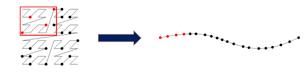
Fortunately, there is already a type of transform that describes this operation in mathematics called a “Space Filling Curve” (SFC). Different SFCs have different properties, but they all take an n-dimensional space and describe a set of steps to trace all points in a single sequence.
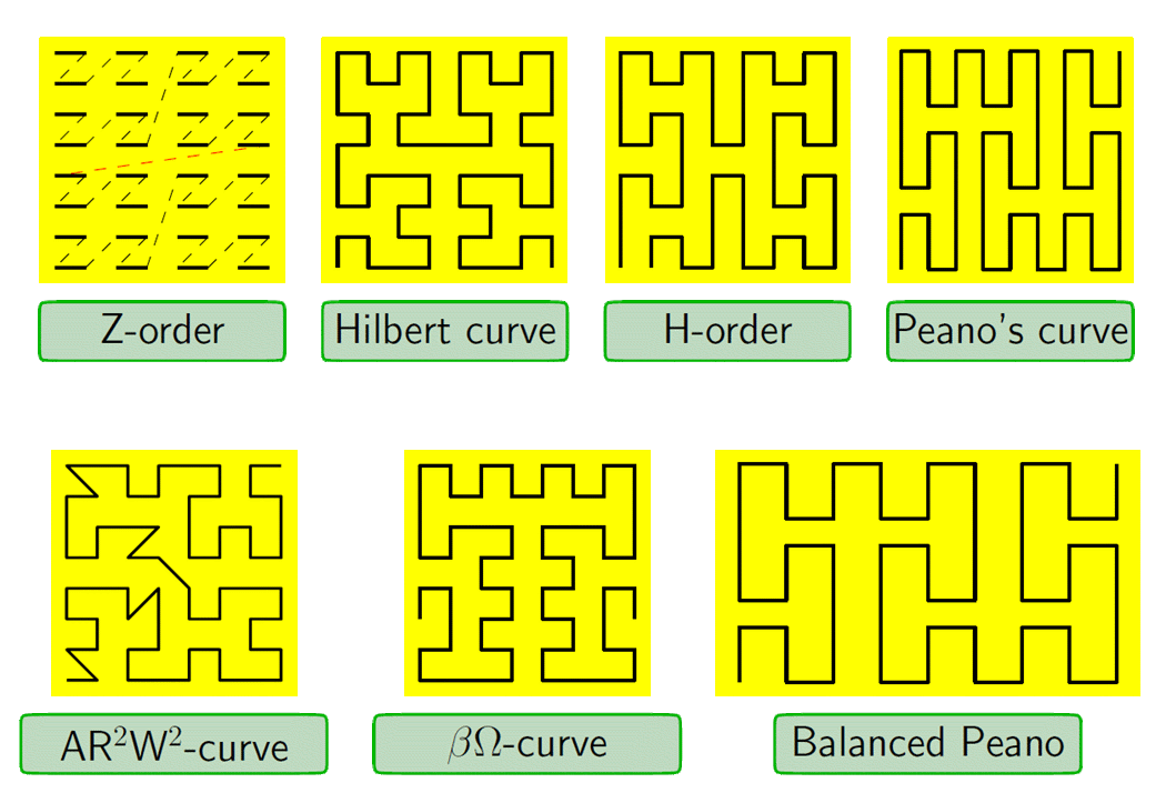
The trade-offs for the various curves are outside the scope of this user manual, but the paper cited for Figure two is an excellent starting point to start learning about these curves.
GeoWave supports two space filling curves: Z-Order and Hilbert, with the latter being the primary implementation.
Hilbert SFC
The Hilbert curve is a bit more complex to work with than the Z-curve, both when calculating and when performing a decomposition. Nevertheless it is popular in certain areas in computer science where multiple variables need to be set in a linear order – process scheduling for one. A simplistic view of a standard projections of the earth mapped to a Hilbert curve would look something like the image below, which shows 4 bits of cardinality per dimension (how many buckets we have).
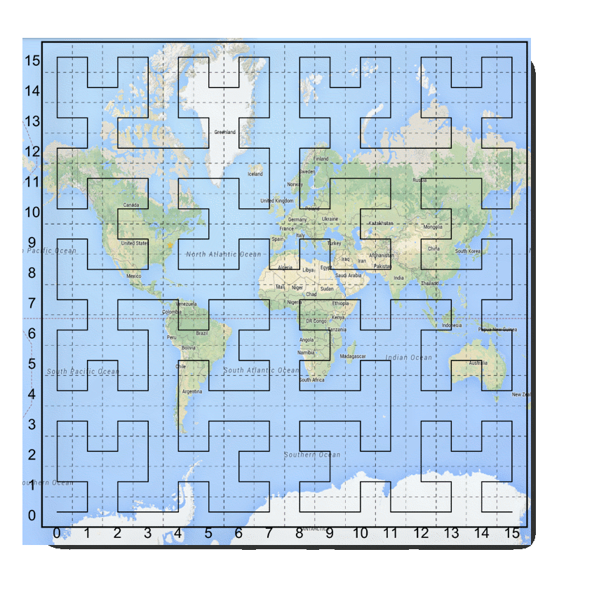
Note that the cardinality (number of buckets per dimensions) has an impact on the resolution of our Hilbert index. Here we map from -180 to +180 over 16 buckets so we have resolution of no better than 360/16, or 22.5 degrees for longitude (and incidentally 11.25 degrees for latitude). This doesn’t mean we can’t represent values more precisely than this. It just means that our initial (coarse) index (based on SFC ranges) can’t provide resolution any better than this. Adding more bits per dimensions will increase the precision of the SFC-based index.
Z-Order SFC
This is also commonly called a GeoHash or Morton order, and sometimes is incorrectly called a Peano curve. This is the most popular SFC used for multi-dimensional → 1-dimensional mappings primarily because it is very easy to implement in code.
To implement this, ideally, a bit-interleaving approach is used (that is what gives rise to the diagram in the figure Z-Order curve based dimensional decomposition). Imagine we had two numbers, A and B. Let the binary representation of those numbers be A1A2A3 and B1B2B3. The “bit interleaved” version would be A1B1A2B2A3B3. Since we are working with binary numbers this gives a “unit cell” of 2x2. If we added dimensions, just imagine the same interleaving, but another term — C1C2C3, etc. This is sometimes implemented in Base 10 instead of Base 2. This implementation somewhat reduces the locality (“packing property” – or the measure of how close numbers in n-dimensional space are to numbers in 1-dimensional space). As you might expect a 2-dimensional version of this gives a unit cell of 10x10 (for two dimensions) – hence the worse packing.
Decomposition
Range decomposition is the core to the concept of SFC-based indexing. This is when we take a range described in multiple dimensions and turn it into a series of 1-dimensional ranges.
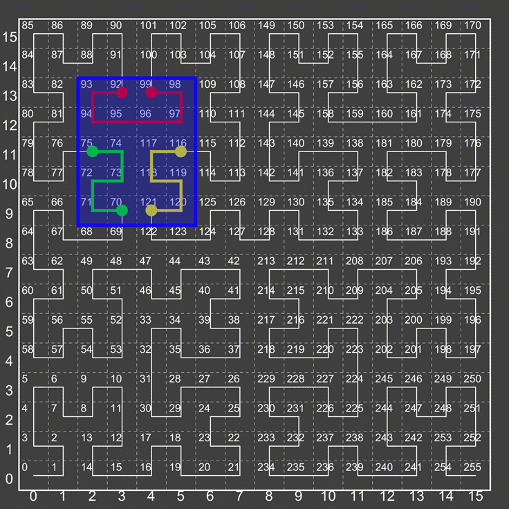
Figure: Hilbert Ranges
In the figure above we show what we mean by this. The bounding box described by the blue selection window, or (2,9) → (5,13), will “fully” decompose to 3 ranges – 70→75, 92→99, and 116→121.
It should be noted that sometimes more simplistic algorithms will not fully decompose, but would instead represent this as 70→121 or even 64→127 (the smallest “unit cell” this box fits in). As you can see, this would result in scanning many extraneous cells.
At some point, with high precision, high dimensionality curves, the number of possible unit cells can become too large to deal with. In such a case, GeoWave optimizes this by treating the curve as a “lower cardinality” curve than it actually is. So the unit cell size might not be 1, but instead 64, 128, 1024, etc. This allows the user to still achieve high precision when selection windows are small but not spend an inordinate amount of time fully decomposing for large selection windows.
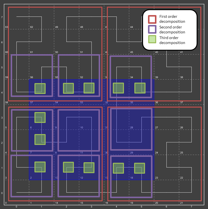
Consider a region query asking for all data from:
(1,1) -> (5,4)
This query range is shown at left by a blue bounding box.
What did we do here?
-
We broke down the initial region into 4 subregions (Red boxes).
-
We broke down each subregion (red box) into 4 sub-sub regions (purple boxes).
-
We then broke down each of those purple boxes into green boxes.
|
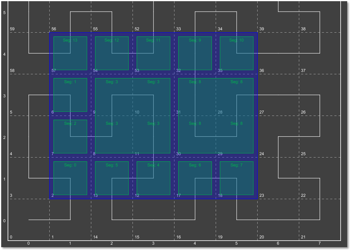
Here we see the query range fully decomposed into the underlying "quads". Note that in some instances we were able to stop decomposing when the query window fully contained the quad (segment 3 and segment 8).
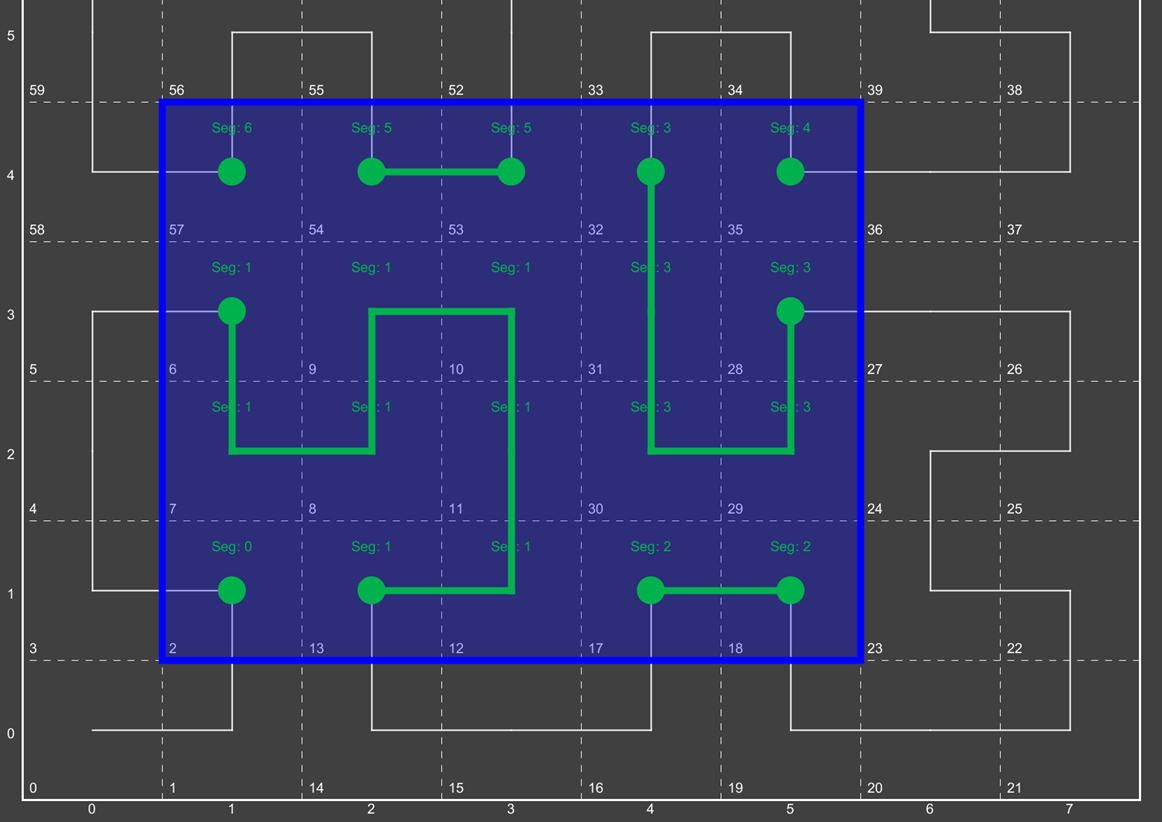
Now we have fully transitioned to the 1-dimensional number line from the previous set of quads. We have also rolled together regions that are contiguous.